|
home
people
research
publications
scholar
SUNTANS
krell fellowships
|
 |
|
Research
Estuarine flow physics and modeling
Model accuracy
The most difficult aspect of estuarine circulation modeling is that
most of the error arises from inaccurate boundary conditions and
forcing, such as bathymetry, river flows, winds, surface waves,
surface heat fluxes, vegetation coverage, and hydraulic structures. As
a result, the underlying model parameters frequently make up for
errors in forcing and boundary conditions at a given grid resolution,
and thus model skill does not always improve with grid
refinement. Therefore, a great deal of our research in this area focuses on
understanding errors resulting from the numerical discretization and
parameterizations versus those arising from the boundary conditions
and forcing.
Although many estuarine models display limited improvement in skill with
grid refinement owing to the aformentioned errors, in some instances it
is possible to improve model skill with grid refinement when the local
errors are dominated by discretization errors. The baroclinic circulation
in North San Francisco Bay is an excellent example (Figure 1). Figure 2 shows
the effect of grid refinement on the error in computing the bottom salinity
at Benicia. The effect of the scalar advection scheme and the turbulence
model (in this case the Mellor and Yamada level 2.5 turbulence closure scheme)
have pronounced effects on the error (Chua and Fringer, 2011). In particular, we don't expect any improvement
in model skill if we employ the turbulence model when first-order upwinding is used.
In this case, the resulting horizontal salinity gradients are so weak due to
numerical diffusion that there is no baroclinic circulation needed to stratify
the water column and impact the turbulence.
Figure 1: Surface salinity in San Francisco Bay over a spring-neap tidal cycle computed
with the three-dimensional SUNTANS model.
Inflows from the Sacramento and San Joaquin rivers totaling 300 m^3/s
drive freshwater oceanward and create the longitudinal salinity gradient in North San
Francisco Bay that arises from a balance between seaward advection by the river flow and landward tidal
dispersion. The inset shows the water level forced at the ocean boundary. No winds or waves
are included. (Setup described in Chua and Fringer, 2011).
Figure 2: Effect of grid refinement on average error between observed and modeled
bottom salinity at Benicia, CA (See Figure 1), over a spring-neap tidal cycle in January 2005.
Four different scenarios are shown to test the
effect of the salinity advection scheme (second-order accurate TVD scheme vs.
first-order upwinding) and the turbulence model (with and without the Mellor and Yamada
level 2.5 scheme). Use of the turbulence model only has an effect when the higher-order
momentum advection scheme is employed because the low-order advection scheme leads to
excessive horizontal diffusion which prevents baroclinic circulation needed to
vertically stratify the water column. Without vertical stratification, the turbulence
model has no effect.
This example of circulation in North San Francisco Bay involved the leading-order
effects of tides and baroclinic circulation.
In many cases, however, we seek results related to high-order or secondary processes
(such as wind-driven circulation, tidal residuals, ocean-driven circulation)
which can be much more difficult to model when both high- and low-frequency processes
are simulated. As an example, the work by Sankaranarayanan and Fringer (2013) in San Francisco Bay shows that
forcing from the Pacific Ocean accounts for less than 5% of the
variance in the currents in Central San Francisco Bay. This implies that model errors in computing
the other dominant processes, such as the tides in the bay, must be
very small if one seeks to model low-frequency effects due to the
Pacific Ocean.
Circulation in a microtidal estuary
|
back to top
|
In much of San Francisco Bay, the tides are the dominant physical mechanism controlling
the circulation given that the averge tidal range is roughly 2 m. However, in microtidal systems like
Galveston Bay, TX (Figure 3), where the tidal range is much less than 2 m,
all forcing mechanisms are of similar magnitude.
Therefore, all must be faithfully computed to obtain reasonable model
skill, including tides, winds, fresh water discharges, atmospheric
heating and cooling, evaporation and precipitation, and possibly,
meso-scale coastal phenomena. At the same time, model validation must separately
validate the low- and high-frequency results to demonstrate model
skill at resolving processes over different time scales. Rayson et al. (2015) showed
this to be an essential component of obtaining accurate SUNTANS
results in Galveston Bay, where, unlike San Francisco Bay, the
low-frequency wind- and Gulf-driven currents account for the same
fraction of the variance as the relatively weak tides.
We used the model of Rayson et al. (2015) to study the complex spatio-temporal variability
of residence times in the Bay (Rayson et al., 2016) as well as an analysis of
the seasonal varibility of the salt flux (Rayson et al., 2017). Figure 4 shows
an example of particle motion in Galveston Bay used to compute Lagrangian residence
times, while Figure 5 shows model prediction of a hypothetical tracer release at the
mouth of the bay.
Figure 3: Map of Galveston Bay, TX. The red dashed region indicates the modeling domain
of Rayson et al. (2015).
Figure 4: Lagrangian particle motion in Galveston Bay, TX, over two tidal cycles.
Each yellow dot corresponds to a particle that can be used to compute the residence time at that location in the Bay,
or the time it takes for tracers to leave the Bay. (From Rayson et al., 2016).
Figure 5: Age concentration from a hypothetical tracer release at the mouth of Galveston Bay, TX. The color
bar is a measure of the relative age of the tracer - "young" tracers have just entered the bay and are relatively
light, while "old" tracers are dark and have been in the bay for much longer.
High-resolution simulations of a macrotidal estuary
|
back to top
|
In contrast to microtidal estuaries, tides dominate the circulation in macrotidal estuaries, which
are defined by a tidal surface range exceeding 4 m. My group studied the salinity dynamics in the Snohomish
River Estuary near Everett, WA, a macrotidal salt wedge estuary. We employed the SUNTANS model with very
high grid resolution in order to understand the impact of complex bathymetric features on the circulation
(Figure 6). Such high grid resolution enables simulation of flow separation around a sill that is exposed
during low tide, as shown in Figure 7. Macrotidal estuaries are
hard to model because of extensive wetting and drying of tidal mudflats,
which imposes strict stability limitations on the free-surface solver in order to
make sure that the water depth remains positive. Additionally, owing to the strong dependence on the
bathymetry, results depend to great extent on accurate bathymetry surveys (Figure 8).
Figure 6: High-resolution, unstructured grid used to model the macrotidal Snohomish River Estuary near
Everett, WA, with the SUNTANS model.
The grid resolution ranges from 300 m at the open tidal boundaries down to 1 m near the
mouth of the Snohomish River. (From Fringer and Wang, 2012).
Figure 7: Surface salinity (in ppt) and velocity vectors (maximum
current is roughly 1 m/s) over a tidal cycle, showing flow separation
around a sill that is exposed during low water in the Snohomish River
Estuary, computed with the SUNTANS model (This region is indicated by the zoomed-in region
in Figure 6). Dark red regions represent exposed
mudflats, while gray regions indicate the water line (the salinity shown is at a depth
that is slightly below the water line). The water level is shown by
the inset in the lower right-hand corner. (From Fringer and Wang, 2012).
Figure 8: Water depth (in m relative to mean lower low water)
during lower-low water, before (left) and after (right) updating
the bathymetry with a high-resolution bathymetry survey. The black regions indicate exposed (dry)
mudflats during low tide, and show how a substantial portion of the domain was still inundated
during low water with the original bathymetry, which was coarse to the west of the red dashed line.
Such inaccurate bathymetry can produce tidal flows that are completely out of phase with the observed tide.
(From Wang et al., 2009).
In addition to accurate bathymetry, accurate predictions of salinity
require a turbulence model to parameterize the effect of turbulence on the vertical mixing of
salt. While a turbulence model is needed to parameterize the mixing,
Wang et al. (2011) analyzed several turbulence closure schemes
and showed that the particular closure scheme (e.g. Mellor-Yamada 2.5, k-epsilon, k-omega, etc...)
is not as important as the stability function, which parameterizes the effect of the stratification
and shear on the mixing. Figure 9 shows transects of the salinity and turbulent kinetic energy
during flood tide along the Snohomish River. The results show little difference among the turbulence
models, but a pronounced effect of the stability function. In this case the stabiilty function
can overdamp the turbulence and lead to less vertical mixing and an overprediction of the upstream
salt flux.
Figure 9: Salinity (left) and turbulent kinetic energy (right) along transect E-E' in Figure 6
during flood tide, computed using the SUNTANS model with different two-equation turbulence closure
schemes and stability functions. The turbulence closure schemes
include k-kl, or the Mellor and Yamada level 2.5 scheme, k-epsilon, and k-omega.
KC and CA correspond to two types of stability functions (Kantha and Clayson, 1994, and Canuto et al. 2001)
that parameterize the effect of stratification and shear on the mixing. The main difference between the
two is the critical Richardson number above which stratification damps turbulence. Because the KC stability function
has a lower critical Richardson number, then turbulence can be generated with the CA
stability function with a magnitude of shear that is lower than what would be needed to generate
turbulence with the KC stability function. The result is overprediction of the stratification and
intrusion of the salt wedge with the KC stability function (Compare Figure 9 a and e to Figure 9 d and h), leading to a more
accurate prediction when using the CA stability function.
Hydrodynamics of salt marshes is unique from a modeling perspective because it requires modeling of the
usual estuarine processes in addition to drag by extensive vegetation and, as is typically the case in
salt marshes in urban areas, engineered structures such as culvert pipes. Vegetation drag and engineered
structures play essential roles both in the hydrodynamics and sediment transport in salt marsh estuaries.
Understanding and modeling of these processes is important for developing informed management
strategies for salt marsh restoration and sustainability.
My group has added new modules to the SUNTANS model in order to study the hydrodynamics of salt marsh
estuaries. These include:
- Hybrid grid compatibility: This allows use of arbitrary-sided polygons
on the unstructured grid. As an example, our work in the Castro Cove region of San Francisco Bay
(Figure 10) employs both triangles and quadrilaterals (Figure 11).
Quadrilaterals enable simulation of along- and cross-channel gradients much more accurately and
efficiently than triangles. Although two triangles can be used in place of a quadrilateral, these
triangles are typically degenerate since the Voronoi points, which are the centers of the circumcircles in
each triangle, either overlap (if the triangles are right), are outside of the triangles (if they
are obtuse), or incur cell centers that are very close together, leading to numerical
stability problems. Regardless of the location of the Voronoi points,
elongated triangles generally lead to inaccurate results.
- Vegetation drag module: This adds momentum sink terms to the right-hand side of the Navier-Stokes
equations to parameterize the effects of the vegetation through a quadratic drag law that takes into
account the flow speed and vegetation geometry, including density, shape, size, etc... To test
the drag parameterization, we used SUNTANS to simulate flow in a laboratory tank with idealized vegetation
with different vegetation heights and densities (Figure 12). The results yield suprisingly good agreement
between the lab experiments and the model (Figure 13). Although the agreement is good, better
agreement in the shear layer could be obtained by including the effects of the vegetation into the
turbulence model. Such effects, however, are less pronounced and even more difficult to calibrate
for field-scale applications.
- Culvert module: To simulate flow through culverts, we implemented the method of Casulli and Stelling
(2013; doi:10.1002/fld.3817),
in which the free-surface is constrained to the top of the culverts when the flow is fully
discharged. A quadratic drag law is imposed in the momentum equations that ensures the correct flow-stage
relationship for the culvert.
- Subgrid bathymetry module: The concept of subgrid bathymetry was developded by Casulli
(2009; doi:10.1002/fld.1896) and enables use of high-resolution bathymetry without needing to
employ high grid resolution. In the method, bathymetry at a resolution that is finer than the grid ("subgrid")
is used to compute the volume and cross-sectional areas of
the finite-volume cells when computing conservation of volume (i.e. the free surface) and mass (i.e.
salt, heat, sediments). In this manner, the cross-sectional areas of the cells match the physical
cross-sectional areas based on the bathymetry regardless of the grid resolution. The
effect of the subgrid bathymetry is also included in the momentum equations and can reproduce
the correct flow-stage relationship in simple channel cross sections when the momentum balance is
predominantly between the barotropic pressure gradient and bottom friction. In channels with
strong lateral variability, lateral momentum fluxes can disrupt this balance, an effect that can be
alleviated by increasing the lateral grid resolution so that the method relies less on the subgrid
reconstruction of momentum. Application of the subgrid method to sediment transport is discussed
here.
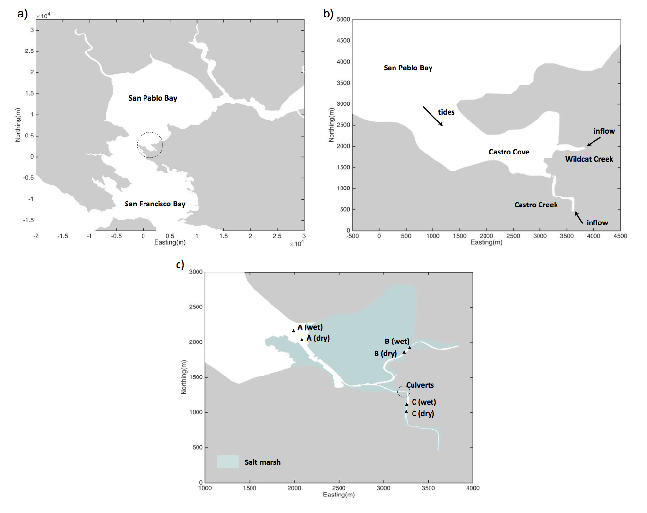
Figure 10: Map of the Castro Cove region (b) which is on the southern end of San Pablo Bay, CA (a), where
we are studying sediment transport in a salt marsh. Panel (c) highlights the extensive vegetation
coverge in green as well as the location of the culverts that were installed to restrict sediment
erosion from Castro Creek. The letters indicated locations of moorings during two (wet and dry)
observational periods.
Figure 11: Unstructured grid of the Castro Cove region with zoomed-in views highlighting the use
of quadrilaterals to resolve narrow channels. The narrow channels in (c) represent the culvert pipes.
Note the presence of quadrilaterals sparsely distributed throughout the triangulated regions, where quadrilaterals
are needed to eliminate obtuse or right neighboring triangles.
Figure 12: Top and side views of the laboratory experiment used to validate the vegetation drag
module in SUNTANS with an idealized array of circular cylinders to represent the vegetation.
Here, Q is the flow rate, hv is the vegetation height, W is the tank width, and D is the depth.
Measurements were taken at location A and compared to the model in Figure 13. Lab experiments
courtesy of Franco Zarama and Itay Rosenzweig at the
Bob and Norma Street Environmental Fluid
Mechanics Laboratory.
Figure 13: Comparison of modeled (dotted) to measured (solid) velocity profiles at location A
within the patch of vegetation in Figure 12. The horizontal dashed line indicates the height
of the vegetation. The agreement is good, although the model underpredicts the strength of
the shear owing to inaccurate representation of the effect of the vegetation drag on the turbulence.
Such effects are not as important in field-scale applications.
|
|
|
Last updated:
05/28/23
|