
A key challenge yet to be addressed by miniaturized bioanalytical devices is the detection of analytes with nanomolar or lower initial concentrations in volumes of one microliter or less. Temperature gradient focusing (TGF) is a promising field gradient focusing technique that simultaneously concentrates and separates charged species according to their electrophoretic mobilities.
In general, focusing methods concentrate species to a fixed point in space through the application of a driving force that vanishes at the focus point. A classic example is isoelectric focusing. In isoelectric focusing, charged molecules or particles move within a pH gradient via electrophoresis. They continue to move until they reach their pI point, at which point their charge is neutralized and they no longer experience an electric force. With field gradient focusing methods, a gradient in electric field causes a change in the electric body force, but the driving force never disappears, and an electrophoretic velocity remains. In this case, focusing occurs where the sum of the electrophoretic mass flux and opposing advective flux equal zero.
Creating an Electrophoretic Flux
Gradient
The viscosity of aqueous buffers decrease significantly
with increasing temperature. As a result, the electrophoretic mobility of
ions increases with temperature, since they experience less viscous drag.
When an axial temperature gradient is applied along some portion of a
microchannel, we have the following:
where m is viscosity and n is ion mobility. The conductivity of a buffer with strong electrolytes is proportional to the sum of the product of each ion’s concentration and mobility. Therefore, the conductivity is inversely proportional to the viscosity, through the temperature dependence of the mobility. This relationship is described by the empirical formula known as Walden’s Rule.
| Walden’s Rule: |
Many common buffers behave according to Walden’s rule. However, buffers with weak electrolytes or reacting components will generally violate Walden’s rule, since the equilibrium dissociation or reaction constants are typically temperature dependent. If we describe the deviation from Walden’s Rule using a function, f(T), we get the following axial conductivity dependence:
where,
|
Given that the electric current flux through the microchannel is approximately conserved at all points, the local electric field is determined by Ohm’s law to be inversely proportional to the conductivity.
Here we see that if the buffer follows Walden’s rule (dotted line), we achieve a gradient in electric field, but no change in electrophoretic velocity (nE), since the mobility and the field vary inversely. However, if Walden’s rule is violated, the electrophoretic velocity will change as a function of temperature. Therefore, by using a buffer with a temperature-dependent ionic strength, and opposing the electrophoretic motion with a bulk fluid flow of appropriate magnitude, we can focus a charged specie to its zero velocity point.
Dispersion in TGF
Dispersion is an important consideration in
microfluidic separation systems. Minimizing dispersion improves separation
resolution, increases the effective detection sensitivity, and improves the rate
of focusing. Dispersion in TGF results from a combination of molecular
diffusion and advective dispersion, as depicted in the schematic below.
Advective dispersion is caused by both externally-imposed and
internally-generated pressure gradients, and its effect may be seen in the
curvature of the focused sample shown with the schematic.
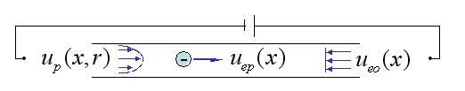
The transport of a charged solute is modeled by the convection-diffusion equation. Here we give the convection-diffusion equation for a circular channel. We have written the equation in a non-standard form to emphasize the fact that only the pressure-driven flux contributes to dispersion through its radial dependence.
Note, in this formulation, up may vary due to internal pressure gradients generated by changes in the electroosmotic flow, but the sum of up and ueo is constant due to continuity.
Experimental Setup
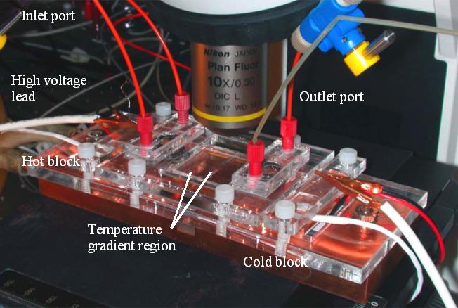 |
| Figure1. TGF experimental setup. The TGF assembly provides the thermal, fluidic, and electrical interface to the microchannel. The microchannel is a borosilicate capillary mounted on a microscope slide or coverslip and embedded in PDMS (for thermal and electrical insulation). A temperature gradient is established across a gap between two copper plates, each heated or cooled by a thermoelectric (Peltier) device. Pressure control is accomplished by adjusting the relative heights of two external reservoirs. |
Temperature Gradient Verification
To quantify the temperature field in our channels, we
performed a set of temperature field measurements by imaging rhodamine B (see
below). We relate these rhodamine intensity measurements to temperature
field data using the method described by Ross et al.
|
Raw image of temperature-dependent rhodamine B fluorescence intensity at l= 580 nm.
|
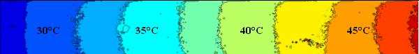 |
Contour plot of processed temperature field showing 2.5°C isotherms. |
Focusing Visualizations
|
False color image of negatively charged bodipy dye in 900mM Tris-borate buffer. The focusing occurred in the thermal gradient shown above with E = -40 V/mm and l = 530 nm. |
(Mouseover figure to begin movie)
Movie shows unsteady focusing of Bodipy dye in an applied temperature gradient of 10 ˚C/mm and applied electric field of -50 V/mm. Pressure head supported the left-to-right electrophoretic flux.
 |
|
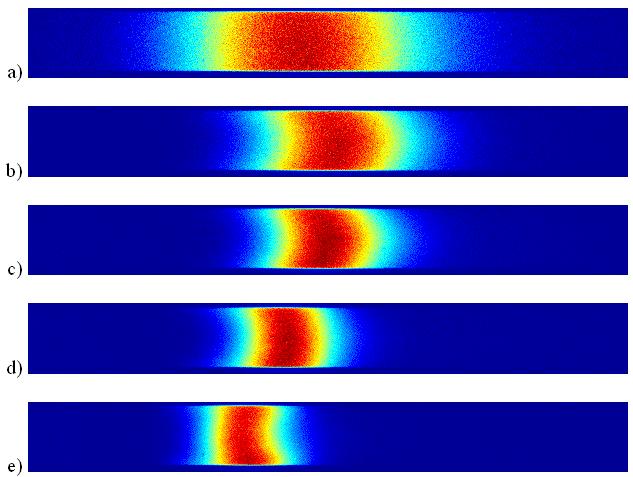
Full field fluorescence images of focused Bodipy dye. The images show the focusing of negatively charged Bodipy dye within the temperature gradient region of a 20 x 200 mm rectangular capillary. The applied temperature gradient was 10 ˚C/mm and the applied electric fields and heads were a) -5 V/mm, 3 mm, b) ‑20 V/mm, 4 mm, c) ‑40 V/mm, 9mm, d) ‑60 V/mm, 15mm, and e) ‑80 V/mm, 22mm. The net flow is right to left, driven by electroosmosis. The pressure head supports the left to right electrophoretic flux. |
 |
|
Temporal development of concentration distribution. The applied temperature gradient was 60 C/mm and electric field was -80 V/mm. The profiles were generated by averaging a 16 pixel wide strip centered on the axis of the channel. Superposed on the data are profiles from a quasi-steady dispersion model. The inset shows the constant growth rate of peak area (which is proportional to the number of molecules collected). |
(Mouseover figure to begin movie)
Movie shows unsteady focusing of four eTags in an applied temperature gradient of 25 ˚C/mm and applied electric field of -80 V/mm. Pressure head supported the left-to-right electrophoretic flux.
References
1. Ross, D. and L.E. Locascio, “Microfluidic Temperature Gradient Focusing,” Analytical Chemistry, 47, pp. 2556-2564.
2. Ross, D., Gaitan, M., and L.E. Locascio, “Temperature Measurement in Microfluidic Systems Using a Temperature-Dependent Fluorescent Dye,” Analytical Chemistry, 73, pp. 4117-4123.
“...transmitted through omnipresent luminiferous diathermanous ether. Heat (convected) ... was constantly
and increasing conveyed from the source of calorification to the liquid contained in the vessel.”
Ulysses, Episode 17: Ithaca, by James Joyce
|