How much is an apple tree "worth" in our economy? Such a question is best interpreted as "how many present units of the numeraire should be traded for the apple tree?". The answer is found by calculating the cost of obtaining the same set of payoffs in another way. The result is the present value of the apple tree. The process of determining the present value of a security or productive investment is termed valuation.
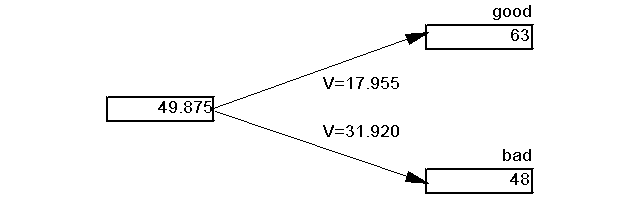
In principle, the process is very simple. Recall that the tree will provide 63 apples if the weather is good and 48 if it is bad. Dealer G will provide the former for 0.285*63=17.955 present apples. Dealer B will provide the latter for 0.665*48=31.920 present apples. The total cost of obtaining the same results in this other manner will thus be 17.955+31.920=49.875 present apples. This is the present value of the apple tree, as shown in the figure below.
There is nothing metaphysical about this concept of value. It is based entirely on the cost of obtaining a fully equivalent set of payments. If an apple tree is selling for less than this, one can obtain an arbitrage by buying the tree and selling its production through the dealers. If a tree is selling for more, one can offer the same outputs, sell them and use the proceeds to buy securities from the dealers to guarantee delivery. In each case, there will be something left over for the arbitrageur.
In real markets, such opportunities are few and fleeting. In an arbitrage-free market, they are totally absent -- there is one set of atomic security prices and every security will sell for a price equal to its present value, computed using these atomic security prices. In such a market the present value of any set of claims is computed by multiplying the quantity of each claim by its price, then summing.
A distinction is often made between the present value and the net present value of a set of claims. The former is generally based on all future payments and thus determines the present value of those payments. The latter is generally based on all payments, including any required payment in the present ("up front"). Thus:
net present value = present value - present payment
In matrix terms, either concept can be represented as equal to p*q where p is a {1*states} vector of elemental security prices and q is a {states*1} vector of payments. In this case, if:
p:
        good weather   bad weather
               0.285         0.665
and q:
   good weather     63
   bad weather      48
then pv = 49.875.
If the tree could be purchased for 49.875 apples:
p:
       present    good weather   bad weather
        1.000         0.285         0.665
and q:
   present         -49.875
   good weather     63
   bad weather      48
and npv = 0.0.
The net present value of an investment that is valued correctly ("fairly priced") is zero, as in this case.
The goal of an arbitrageur is to find a strategy with a positive net present value. As indicated earlier, arbitrages are hard to find in well-developed capital markets.
How can an entrepreneur evaluate a "trade with nature" (productive investment)? If the commodities produced by such activity will not significantly alter either commodity prices or time-state-claim prices, the rule is simple: engage in any such investment with positive net present value.
Assume that a scientist discovers how to plant 60 apples in a way that will produce 100 apples if the weather is good and 50 apples if the weather is bad. Is this desirable? To find out, compute the net present value:
p:
       present    good weather   bad weather
        1.000         0.285         0.665
q:
   present          -60
   good weather     100
   bad weather       50
and npv = 1.75. The NPV is positive, so the technology should be implemented.
The entrepreneur might sell stock in this apple firm. Its value would be 61.75 apples, which is the present value of the possible future payments. Thus the scientist's investment of 60 apples could be turned into 61.75 apples today. She could (1) use the profit of 1.75 apples today, (2) swap it for apples next year if the weather is good, (3) swap it for apples next year if the weather is bad, or (4) select some combination of the three alternatives.
In practice, of course, it is not always easy for an insider to cash in on the future prospects of his or her enterprise. Our example assumes that outside investors are able to confirm that the scientist's tree will in fact produce 100 apples if the weather is good and 50 if the weather is bad. Security analysts, who study publicly-traded securities, attempt to make the best possible forecasts of firm's future prospects and the associated payments to the holders of their securities. Banks and other credit-granting agencies expend substantial resources to assess the firms to which they may lend money. And, of course, the managements of companies provide information about their progress and prospects. However, there is the ever-present possibility that insiders may provide forecasts that are overly optimistic, either through excessive enthusiasm or in an attempt to drive up the prices of securities that they may wish to sell.
The underlying problem is the fact that the parties to a proposed trade may have different sets of information. The possibly negative effects of the resulting asymetry can be mitigated in a number of ways. Insiders may retain substantial positions in a firm to show their good faith. They may pledge their personal assets to cover certain types of shortfalls. And so on. At the very least, however, additional resources will be almost certainly have to be expended to verify predictions, audit records, etc..
In our quest to establish first principles in a simple setting, we leave until later an extended discussion of issues associated with differential information, the costs associated with attempts to improve participants' information sets, etc.. For now we assume that people agree on the payment vectors associated with various investments and that the only source of uncertainty concerns the state of the world that will actually obtain.
A riskless security pays the same amount at a given time, no matter what state of the world obtains. Equivalently, it is a bundle of equal amounts of atomic claims for a time period. In our case, a riskless security pays a fixed amount (say X apples) at time period 1, whether the weather has been good or bad. Equivalently, it is a bundle of X good weather apples and X bad weather apples.
To value such a security one follows the general rule: multiply price times quantity. For example, assume that a AAA-rated security promises to pay 20 apples at time period 1. Then:
p:
       good weather   bad weather
           0.285         0.665
q:
   good weather     20
   bad weather      20
and pv = 19.00.
Note that this computation involves multiplying a fixed amount (20) by each of the atomic security prices for claims for the associated date, then summing the results. One could as well have summed the prices, then multiplied the result by the fixed payment. In this case:
  (0.285 * 20) + (0.665 * 20)
        =    (0.285 + 0.665) * 20
        =    0.95 * 20
The sum of the appropriate atomic security prices is termed the discount factor for the date in question. It represents the present value of a payment of one unit to be made with certainty at the specified future date. The process of computing a present value in this manner is called discounting. Thus one discounts the (certain) future value to obtain the present value of a riskless security.
Note that this calculation, like any other valuation analysis, rests on the ability to obtain the same set of payments in a different way. An apple a year from now has a present value of 0.95 apples because one can obtain the same thing using other types of transactions. Absent functioning markets that provide alternatives, the processes of valuation (in general) and discounting (in particular) lack a rigorous basis.
In an arbitrage-free economy with no transactions costs, any given time-state claim will sell for the same price, no matter how obtained. This will also be true for any "package" of time-state claims. This property is known as the law of one price.
It is easy to see why the law must hold in an economy of the sort we have posited. Assume that a given set of time-state claims can be traded for cash today at either of two prices -- X or Y. Then an arbitrageur could buy the set of claims for the lower of the two prices and sell it for the higher, pocketing the difference. No matter what occurred in the future, he or she would receive from one counterparty exactly the cash required to meet the promises made to the other.
In the real world where transactions costs are relevant, the lack of arbitrage opportunities only insures that prices for a given set of time-state claims will fall within a band narrow enough to preclude transactions that can provide something for nothing net of transactions costs. Moreover, since different traders face different transactions costs, it may be possible for some to make money from discrepancies in prices, while others cannot.
Traders, financial institutions, and those who create new financial instruments attempt to exploit discrepancies in prices that arise from transactions costs, broadly construed. In so doing, they may make money for themselves. But they also tend to decrease the transactions costs that will be borne by others. Thus the actions of arbitrageurs and other traders tend to bring markets for key time-state claims and combinations of such claims closer and closer to the ideal of zero transactions costs and true conformity with the law of one price.
We return now to our "standard" apple tree, which will produce 63 apples if the weather is good and 48 if the weather is bad.
Consider an entrepreneur who wishes to set up a firm that will buy one such tree. As we have shown, the present value of the tree is 49.875 (present) apples. To buy the tree, our entrepreneur thus needs 49.875 apples. How can he get them?
One alternative is to simply take it out of his bank account, borrow money on his house, etc.. In such a case, he will serve as both owner and manager.
To keep things simple, we assume that the firm has no costs. Hence its revenues will equal its profits (revenues minus costs). Since our world ends at the end of the year, the firm can be also be expected to distribute these profits.
If the entrepreneur provides all the financing, the firm can provide him with a security that provides the holder with the property right to receive all the earnings that it distributes. Such an instrument would be termed an equity security or, more commonly, a common stock. In this case, the firm can be said to have employed an all-equity financing strategy.
In practice, the firm might issue 100 stock certificates, each representing the right to receive 1/100'th of the firm's distributions. Each certificate would be called a share of the firm's stock. The holder of one share would receive 0.63 apples if the weather is good and 0.48 apples if the weather is bad. Not surprisingly, one share would be worth 0.49875 present apples -- 1/100'th of the value of the set of all outstanding shares.
But there are other ways to finance a firm. In fact, the possibilities are almost endless. We consider first a simple example involving two classes of securities.
Assume that the firm issues a bond of the following form:
    The Apple Tree Firm promises to pay the holder 20 apples
    at the end of the year, no matter what the weather has been
and a stock of the form:
    The Apple Tree Firm promises to pay the holder all the
    apples left over after the bondholder has been paid.
The stock is a residual claim, while the bond is a prior claim -- it is senior in the firm's capital structure.
What is the bond worth? What is the stock worth?
First, the payment vectors.
qfirm:
   good weather      63
   bad weather       48
qbond:
   good weather      20
   bad weather       20
qstock = qfirm - qbond:
   good weather      43
   bad weather       28
It is straightforward to compute the values:
   p*qfirm   =  49.875
   p*qbond   =  19.000
   p*qstock  =  30.875
In the previous example the sum of the values of the securities equaled the value of the firm. This is not too surprising. The payments made by the firm are simply divided among the claimants:
qbond + qstock = qfirm
But thus it must be the case that:
p*(qbond + qstock) = p*qfirm
and:
p*qbond + p*qstock = p*qfirm
Spelled out:
value of bond + value of stock = value of firm
The result is perfectly general. No matter how the payments are divided among claimants, the sum of the values will be the same. This is known as the principle of value additivity.
While it is entirely possible to help one set of claimants and hurt others by rearranging the allocation of cash flows among them, the sum of the values should be unaffected by any such allocation. More simply put, financial decisions that only redistribute claims should not affect total value. Some characterize this as the principle of the conservation of value.
It is, of course, important to include all the claimants in such calculations. In the real world, governments impose taxes on firms and/or those who receive income from firms. As a result, the government must be included when considering claimants to a firm's cash flows. Moreover, lawyers, accountants, investment bankers and others are likely to absorb more of a firm's proceeds under some financial arrangements than under others. Thus while total value may be conserved, some financial legerdemain may divert substantial amounts of value from prior claimants towards those who aid in a transformation.
The principle of value additivity assumes that prices of time-state claims are unaffected by any changes in the financing of the firm. If a proposed change is large relative to the underlying set of associated time-state claims in an economy, it may be necessary to take into account alterations of time-state claim prices and any resulting increases or decreases in value.
If financial arrangements actually affect a firm's operations and hence its revenues and/or costs, value may in fact be increased (or reduced) as well as re-distributed. Some have argued that greater ownership by managers and/or greater debt burdens may increase managerial incentives to maximize profit and hence increase overall firm value. The possibility of such effects is generally accounted for outside the domains of standard valuation theory.
A bond represents debt in which a borrower promises to pay a lender specified amounts in the future. More precisely, the borrower promises to pay if he or she can. If the borrower is a corporation with limited liability, the payment will be made in full and on time only if the borrower's cash inflows and cash outflows associated with claims with greater priority permit. Otherwise, some or all of the promised payment will be in default (i.e. not paid).
Consider an owner of one of our apple trees who issues a bond that promises to pay 60 Apples in period 1 (if possible). If the weather turns out to be good, the payment will be made in full. If it turns out to be bad, only 48 Apples will in fact be paid.
The valuation of such a bond is shown below.
                                    Present
      State     Payment   Price      Value
       good        60     0.285      17.10
       bad         48     0.665      31.92
                                   --------
                                     49.02
Note that the bond will not sell for as much as a similar bond that is riskless. The latter would sell for 60*0.95, or 57 present apples. Comparing the promised payment with the present value (price of the bond) will favor the risky bond (60/49.02) over the riskless one (60/57). It is not surprising that risky bonds offer higher promised yields than riskless ones. A more difficult question concerns their expected yields, taking the possibility of default into account. We deal with these issues subsequently.
The presence of risky debt does nothing to affect the principle of value additivity. Consider the prospects of the residual claimants (stockholders) in this case:
                                    Present
      State     Payment   Price      Value
       good         3     0.285      0.855
       bad          0     0.665       0
                                   --------
                                     0.855
The sum of the values of the bond and stock claims will be 49.02 + 0.855, or 49.875, which equals the value of the underlying assets (the apple tree).
One of the problems associated with financing via two or more classes of claims is that of avoiding decisions that may increase a firm's value but actually decrease the value of one or more set of claims. A simple example can illustrate the point.
Consider the apple tree firm that has bonds outstanding with promised payments of 60 apples. As shown earlier, the value of the firm is 49.875, divided between the value of the bonds (49.02) and that of the stocks (0.855). Now, assume that management has an opportunity to trade its present apple tree for one that will produce 61 apples if the weather is good and 49 apples if the weather is bad. The value of this new tree is shown below:
                                    Present
      State     Payment   Price      Value
       good        61     0.285      17.385
       bad         49     0.665      32.585
                                   --------
                                     49.970
Clearly the proposed trade is desirable, since it will increase value from 49.875 to 49.970. But this new value will be distributed differently:
               Before        After
    Bond        49.020      49.685
    Stock        0.855       0.285
               --------     ------
                49.875      49.970
While the value of the firm has increased, the value of the stock has actually decreased! The increase in the bond's value due its greater security has swallowed more than the entire increase in the value of the firm. While those holding bonds (or even proportional amounts of bonds and stocks) would endorse the change, those holding only stock would be violently opposed.
In principle, stockholders and bondholders in such a situation could work out a re-arrangement of terms to their mutual advantage so that such an opportunity could be exploited. However, this may require time, bargaining, legal costs, etc., making the cost greater than the benefit.
In this case a change in the firm's business to one of lower risk advantaged holders of (formerly) risky debt and disadvantaged holders of junior claims (here, stock). In the converse situation, an increase in the risk of a firm's operations may lower the value of bonds and increase the value of stock. Such a change may not enhance the firm's total value, but may still prove desirable for stockholders. To minimize temptations on the part of management to engage in such tactics, bondholders typically require covenants placing at least some restrictions on management prerogatives. The danger, of course, is that profitable (value-enhancing) undertakings that may increase risk will be foregone as a result.
Thus far we have assumed that dealers stand ready to buy and sell atomic securities that pay off in one and only one time and state of the world. This is not totally fanciful, for financial instruments with similar characteristics do exist. For example, a term life insurance policy will provide payment only if the state of the world is "insured is dead". Conversely, an annuity policy will provide payments only if the state of the world is "insured is alive". Indeed, one could (at great expense) provide a riskless security by purchasing both a life insurance policy and an annuity. Nonetheless, it is true that the typical traded security is better characterized as a bundle of different types of time-state claims. Does this obviate our approach? In principle, no.
Imagine a world in which only two securities are traded on a regular basis. One is the common stock of the Apple Tree Firm described above. The other is its bond. It is convenient to represent their payments in matrix form.
Let Q be:
                 Bond   Stock
  Good Weather    20      43
  Bad Weather     20      28
Assume that the bond sells for 19 Present Apples and that the stock sells for 30.875 present apples. The vector of security prices is thus:
ps:
     Bond       Stock
      19        30.875
Consider now the payoffs obtained from a given combination of securities, for example, a portfolio that includes 1 bond and 2 stocks. We represent this is a vector of the number of each type of security. Here,
n:
   Bond      1
   Stock     2
To determine the number of apples provided by this portfolio in each state of the world we multiply Q by n to obtain c, a vector of payments. (We utilize c to indicate cash flows, even though a might be more appropriate here, given the fact that apples are involved).
As always, it is useful to check to see that the dimensions are appropriate. Here:
Q {states*securities} * n {securities*1} ----> c {states*1}
This operation can be performed regardless of the number of securities. In this case we have as many securities as states; however portfolios with fewer securities than states or with more securities than states can be used in the calculations as long as the requisite information is contained in both Q and n.
In this case, the resulting set of state-contingent payments is:
c:
   Good Weather     106
   Bad Weather       76
Note that in these calculations we started with a portfolio, n, then computed the resulting contingent cash flows (payments), c. We turn now to the reverse question.
Assume that one wishes to obtain a set of state-contingent payments c. What portfolio n will provide them? As before, the requisite equation is:
Q*n = c
If Q is square, it may be possible to take its inverse. If so:
n = inv(Q)*c
and this relationship can be used to determine the portfolio n that will provide a desired set of state-contingent payments c.
For example, assume that one wishes to have 845 apples if the weather is good and 620 if the weather is bad, i.e.
c:
    good weather   845
    bad weather    620
then: inv(Q)*c =
     Bonds      10
     Stocks     15
How much will this portfolio cost? To find out, we "price it out" by multiplying the vector of security prices times the portfolio positions:
ps*n = 653.125
It will cost 653.125 present apples to provide the desired contingent payments (845 apples if the weather is good and 620 if the weather is bad). One way to do this is to purchase 10 Apple Firm bonds and 15 Apple Firm Stocks.
Note that in the above calculations:
ps*n = ps*inv(Q)*c = [ps*inv(Q)]*c
The bracketed expression is of particular interest. In this case it is:
   ps*inv(Q) =
              0.285   0.665
This should look familiar. It is, in fact, the vector of atomic state prices with which we started. This is not surprising, since the cost of any vector of state-contingent payments can be found by multiplying this vector times the desired payment vector. In the special case in which c has a one in the first row and zero in the second, the answer will be 0.285. But this is the cost of an atomic claim in state 1 (good weather). Similarly, if c has a zero in the first row and a one in the second, the answer will be 0.665 -- the cost of an atomic claim in state 2 (bad weather). The result is quite general:
p = ps*inv(Q)
Even in a market in which atomic securities are not traded explicitly, it is possible to create them synthetically by combining positions in existing securities. Moreover, any desired set of payments can be replicated with a suitably-chosen portfolio of existing securities. The cost of obtaining that set of payments can be determined by computing the cost of the replicating portfolio. Equivalently, it can be determined by pricing the contingent payments using the atomic security prices implicit in the prices of existing securities.
Note that this bit of apparent legerdemain requires the inversion of Q -- the matrix that maps securities to payments in states of the world. For this to even be possible, Q must be square -- there must be precisely as many securities as states of the world. In addition, the securities must be sufficiently "different" that an inverse can be computed. If both conditions are met, the securities represented in the matrix can be said to span the space of time-state payments.
What if there are more securities in the world than there are states? Simple. If there are M states, select M (different) securities for inclusion in matrix Q, then compute the implied atomic security prices. Next, for each remaining security: compute the present value using the derived set of atomic prices and compare the result with its traded price. If there are no discrepancies, the market is arbitrage-free and the computed atomic prices can be used for all further calculations. If you find a discrepancy, it is possible to get something for nothing via arbitrage with a set of trades involving the securities in Q and the security for which the associated value differs from price. Stop everything and take advantage of this information. Then, when you have helped bring markets back to an arbitrage-free status (and reaped your reward for undertaking this socially valuable activity), proceed with the analysis as above.
Imagine an investor who tells an investment banker that he would very much like to receive 100 apples next year if the weather is good, and 130 if it is bad. His question: how much will the investment banker charge to guarantee that her firm will provide such payments?
To find the answer, we set c:
    good weather   100
    bad weather    130
then compute:
n = inv(Q)*c:
     Bonds     9.30
     Stocks   -2.00
and:
ps*n = 114.95
If the client will pay at least $114.95, the investment banker can provide the commitment and make a guaranteed profit. Perhaps she will quote $120.00. If the client accepts, the banker can purchase 9.30 apple firm Bonds and short 2.00 of its Stocks. This will cost $114.95, leaving $5.05 in profit. However, the investment banker is perfectly hedged. No matter what the future state of the world may be, her payments to the client will be exactly offset by the net receipts from the portfolio.
Specialists who make such computations are termed financial engineers. Their task is to determine ways to provide desired sets of payments under various contingencies with existing securities and/or new arrangements that can partially or fully offset other commitments.
Given an initial wealth and a set of market opportunities, an investor can attain a number of alternative combinations of time-state claims. The set of all such opportunities is termed (rather unimaginatively), the investor's opportunity set.
To separate the influence of wealth from that of market opportunities, one can consider the set of opportunities available with a wealth of one unit of present value. A particular investor's opportunity set will have the same form, scaled up as needed to account for his or her wealth.
In the present instance we can plot such a set as a three-dimensional diagram since there are only three needed dimensions -- present apples, good weather apples and bad weather apples. We do so in a later section. For now we consider an even simpler case that focuses on the opportunities for future apples per present apple invested.
We plot four investment strategies. The first represents purchase of a pure "bad weather apple" security, the second one of the Apple Tree Firm's bonds, the third one of the firm's stocks, and the last a pure "good weather apple" security. The associated payment matrix is:
Q:
                   Good Bond Stock Bad
   Good weather     1    20   43    0
   Bad weather      0    20   28    1
and the associated security price vector, ps is:
          Good    Bond    Stock      Bad
         0.285   19.000   30.875    0.665
We wish to determine the future apples per present apple invested for each of these securities. To do so we divide each future value in Q by the corresponding price in ps:
 q ./ [ps;ps] =
                 Good     Bond      Stock     Bad
 Good Weather   3.5088   1.0526    1.3927      0
 Bad Weather       0     1.0526    0.9069    1.5038
The ratio of an ending value to the initial value is termed a value relative. Thus if the weather is good, the value relative for a stock will be 1.3927. Subtracting 1.0 gives the return. If the weather is good, the stock will return 0.3927, or 39.27 percent. Note that an atomic security will return -100% in all states and times but the one for which it is designed.
All the returns are plotted in the figure below and connected with a straight line:
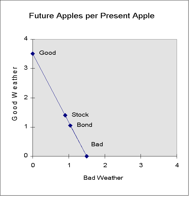
The point representing the bond lies on a line sloping upward at 45 degrees from the origin, since it provides the same payment in each state of the world. The point representing the stock lies above it and to the left. One can attain any combination lying on the straight line connecting these two points by holding a portfolio of both securities, with the sum of the values of the two holdings equal to one present apple. The larger the amount invested in the stock, the closer the point will be to the point representing an all-stock portfolio. The larger the amount invested in the bond, the closer the point will be to the point representing an all-bond portfolio. Let rb be the vector of value relatives for the bond (column 2 in the matrix above) and rs the vector of value relatives for the stock (column 3 in the matrix above). Then the vector of value relatives for a portfolio with proportion xs invested in the stock and (1-xs) invested in the bond will be:
rp = xs*rs + (1-xs)*rb
For example, with xs = 0.6:
   rp =
        1.2567
        0.9652
If only the bond and the stock can be traded, how can one attain points on the line outside the range encompassed by these two securities? Simple. Apply the same formula, but with a negative value of xs or (1-xs). Thus if xs = -0.5 and (1-xs) = 1.5:
  rp=
       0.8826
       1.1255
Since the equation is one of a straight line, any point on the extension of the line through the points representing the two traded securities is available by combining a long (positive) position in one with a short (negative) position in the other. Our two atomic securities are, of course, extreme cases of this general principle.
This example shows graphically why any two securities can be used to "span a space" with two states of the world. It also shows why any security not priced in accordance with the atomic prices implied by two traded securities will present an opportunity for arbitrage. Assume that a third security (Z) exists that plots above the line in the figure. Imagine a line drawn from it to the origin. Label as ZZ the point at which this constructed line crosses the line in the figure. The portfolio of bonds and stocks that will provide ZZ offers a smaller payoff in each state of the world than does Z. Thus one could take a short position in portfolio ZZ and use the proceeds (one present apple) to purchase security Z. In each future state of the world, security Z would provide more than enough apples to pay the counterparty or counterparties to the short position in portfolio ZZ. Voila: something for nothing.
Once arbitrage opportunities of this sort have disappeared all possible strategies will on a linear opportunity set. In a two-dimensional case such as this, the set will plot as a line. In a three-dimensional case it will plot as a plane. In higher dimensional cases the task of plotting would be arduous indeed, but mathematicians would say that the points "plot" on a hyperplane.
If one wishes to be precise, both the linear frontier and all points under it should be considered members of the opportunity set, since one can always throw apples away. The points on the frontier can be said to constitute the set of efficient opportunities, since only individuals who could be satiated (get too much of a good thing) might wish to consider interior points.
Note that all of this discussion depends on the assumption that one can take a negative position in a security when and if desired. This can be done by simply signing a document of the form:
    I promise to pay the holder whatever the Apple Tree Firm
    pays its stockholders
Alternatively, one can engage in a short sale. This is implemented as follows. Assume that A wishes to sell stock X short (equivalently, take a short position). He or she can borrow shares from B, who does own them, then sell them to C (who can remain oblivious to the fact that the shares were never actually owned by A). Upon the sale of the shares, A will receive an amount equal to the price of the shares -- exactly the reverse of the situation that would obtain if he or she had purchased them (in which case A would have paid this amount). However, A will have promised to "make B whole", by paying to B anything that B would have received had he or she retained the shares. In addition, B can usually demand that A return the shares on demand. One way or another, A will pay the amounts that someone who had purchased the shares would have received. Here, too, the situation is reversed. In such circumstances, a short sale will in fact be equivalent to a negative purchase.
In practice, things are not always this simple. B may worry that A will be unable to make some or all of the required payments and/or fail to purchase the stock if and when B calls for its return. Hence B may demand that A earmark some "good faith money" that can be acquired in the event of any such default. Worse yet, B may require that A forego some or all the interest earned on such money, with such gains going to B. Under such circumstances, a short sale is not precisely equivalent to a negative purchase.
Increasingly, institutional arrangements allow investors to take short positions that are very similar, if not identical, to negative holdings. Any costs or impediments associated with such approaches can be considered transactions costs. As usual, we will generally ignore them to avoid even more complexity.
Consider the opportunities available to an individual with W apples to spend. He or she could spend the entire W apples immediately, obtaining thereby W units of consumption today. In this rather extreme case, he or she could look forward to no consumption in the future.
An alternative (and equally extreme) strategy would involve purchase of the maximum number of claims for future consumption if the weather is good. Since the price of each such claim is 0.285 apples, he or she can exchange W apples today for 3.5088*W apples in the future if the weather is good. Of course, such a choice involves zero consumption today and zero consumption in the future if the weather is bad.
The third possible extreme strategy involves the exchange of apples today for the maximum possible amount of consumption in the future if the weather is bad. Since each such claim costs 0.665, a total of 1.5038*W apples can be consumed under these conditions, but only by sacrificing both consumption today and in the future in the event that the weather is good.
These choices are extreme or pure consumption-investment strategies. One and only one type of time-state claim is chosen, with all others rejected. Clearly, few would choose such strategies.
The figure below shows the opportunity set in this case. It is a plane, the borders of which are shown by the three red lines connecting the extreme strategies.
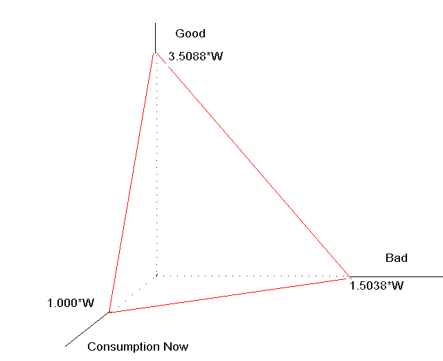
The most interesting alternatives lie on the portion of the plane away from the corners. Such points represent efficient combinations of present and contingent future consumption. Any point on the plane can be obtained by an individual with a wealth (present value) of W apples by a judicious allocation of that wealth among the three "pure" strategies and/or any other securities that are priced appropriately.
Our use of the term wealth in this example is not gratuitous. The wealth of an individual may be defined as the maximum amount of present consumption that could be obtained if all his or her property were sold (traded for present units of the numeraire). Thus an individual who owned an apple tree might currently be located at a point near the middle a plane such as that shown in the figure, but his or her wealth would still be measured by the intercept on the consumption axis of the plane through that point.
Given market prices, individual opportunity sets will differ only in scale. If individual D is twice as wealthy as individual C, her opportunity set will be parallel to that of C but twice as far from the origin. An individual's opportunity set will thus be determined by his or her wealth and security characteristics and prices.
In an economic sense, anyone who chooses a point on the opportunity set other than the one at the all-consumption corner is an investor who sacrifices potential present consumption to obtain at least the possibility of future consumption. The goal of the Analyst is to help the Investor understand the possible trade-offs and then move efficiently from the point representing current opportunities to the point on the frontier of the opportunity set that is most desirable for the Investor.
It is convenient to decompose a set of choices of this sort into a consumption/investment decision and an investment decision. In a three-dimensional diagram, the former would concern the position chosen on the Consumption Now axis, while the latter would concern the relative positions chosen on the Good and Bad axes. While this dichotomy is useful, it is important to remember that investment opportunities may influence one's consumption decision and that consumption opportunities may influence one's investment decision.