Many models of capital market equilibrium are derived from assumptions about the preferences of a so-called representative investor. In essence, security prices are assumed to be set in a manner that would lead to the equality of demand and supply if every investor had such preferences. Some approaches simply assume that every investor has the preferences of the representative investor. Others explicitly model diverse investors and derive the preferences of the representative investor by aggregating the preferences of actual investors. However, even in such approaches, each investor is assumed to have preferences that can be described with a particular type of function, with individuals differing (if at all) only with respect to one or more of the parameters of the specified family..
Practitioners of financial planning do not always use explicit models of investor preferences and financial market behavior, but they tend to advocate investment strategies that are consistent with particular combinations of assumptions. More specifically, financial advisors frequently advocate constant mix strategies, in which the proportions of the value of a portfolio allocated to specific types of assets are kept relatively constant through time. Such an approach is consistent with a particular combination of assumptions about market behavior and investor preferences, but may be inappropriate in other types of markets or for investors with other types of preferences.
This paper attempts to shed some light on the range of preferences of individual investors. It presents the results of a survey of the preferences of 66 respondents, using the Distribution Builder approach developed by Sharpe, Goldstein and Blythe (hence SGB).1
The paper is organized as follows. Section 1 describes the user interface and the key characteristics of the user's experience when taking the survey. Section 2 describes the procedures used to determine the cost of each distribution. Section 3 deals with relevant issues concerning investor preferences. Section 4 describes the key questions addressed in the remainder of the paper. The results of the survey are presented and discussed in section 5. Section 6 concludes and offers suggestions for further research.
The distribution builder approach is designed to let a participant choose a probability distribution of future income that is feasible in the sense that the cost of obtaining the distribution not exceed a fixed budget. The central feature of the user interface is a playing field with a number of rows, each of which can contain markers. In this survey, there are 100 such markers, each of which is represented by a question mark. One of the markers represents the individual, but he or she does not know which one it is. Initially all 100 markers are in a reserve row at the bottom of the playing field. Using controls on the user interface the participant moves the markers into the rows in the playing field and then from row to row, as desired.
Figure 1 shows three rows from the playing field. In this survey each row corresponds to a standard of living in retirement, expressed as a percentage of the participant's income just before retirement. In figure 1 there are 20 markers in the row corresponding to a 75% standard of living, 50 in the row corresponding to a 70% standard of living, and 30 in the row corresponding to a 65% standard of living. Since any marker may be the individual in question, this provides an intuitive understanding of a probability distribution with probabilities 0.20, 0 .50 and 0.30 of retiring with a 75%, 70%, and 65% standard of living, respectively.
Above the playing field is a window with the controls that the participant uses to move the markers on the playing field, a button to be pressed when the preferred distribution is obtained, and a window showing the percent of budget used by the currently chosen distribution, This portion of the interface is shown in figure 2.
For any distribution selected, there is an associated cost, which is expressed as a percentage of the fixed budget. Whenever the user moves one or more markers, this cost is computed, with the new value shown at the top of the user interface. This cost is not the expected value of the probability distribution, but rather the amount of a 100 unit budget that would be required to achieve that distribution using the cheapest possible investment strategy. The participant is not allowed to complete the survey until he or she has selected a preferred distribution that uses between 99% and 100% of the budget with no markers in the reserve row. In this survey the most conservative distribution that uses up the budget is achieved by placing all the people in the 75% row.
After choosing a preferred feasible distribution, the participant is asked to answer the questions about his or her experience shown in figure 3.
The answers to these questions, the time spent and the distribution chosen by the participant are then recorded in a central database, Finally, one of the 100 markers is randomly selected and the user is told which row actually contained his or her marker. This last "revelation phase" is included primarily to make the experience more entertaining, although its presence may lead some participants to focus more on the nature of the probability distribution than they might otherwise.
In this survey there are 100 markers, each of which has an equal probability of representing the participant. The underlying premise is that there are 100 distinct states of the world, each with a probability of 1/100 of occurrence. Moreover, for each state s there is an Arrow-Debreu state price Ps. Thus a present outlay of Ps guarantees a payment of $1 in state s and nothing in any other state. In the user interface, outcomes are expressed as annuity payments measured as percentages of a pre-retirement standard of living, but for computational purposes they can be treated as levels of terminal wealth. Thus a 75% standard of living is considered a terminal wealth of $75.
The participant selects a probability distribution by placing the 100 markers in rows on the playing field. A given probability distribution can typically be obtained in many ways, as long as the wealth level associated with each marker is assigned to one state of the world. We can thus map the user's probability distribution to a vector of wealth levels w1,w2,...w100. The cost of obtaining a given amount of wealth ws in state s will equal Psws while the cost of obtaining the entire vector of wealth levels will be:
C = Ss Ps*ws
While there are many possible mappings of a distribution to states, it is plausible to assume that every participant would prefer to obtain any given distribution in a way that would minimize the cost2. This is easily achieved. First, states are ordered from the lowest to the highest state price. Then wealth levels are assigned to states from the highest wealth to the lowest. This guarantees that it will be impossible to change the assignment in any manner that will decrease cost.
The survey software automatically provides this least-cost mapping from a distribution to a corresponding vector of wealth levels by state. The percent of budget used is computed by dividing the resulting cost by a fixed initial budget, B:
% of budget used = (Ss Ps*ws ) / B
For some purposes it might not matter how the state prices used in the survey are established. However, to make the trade-offs facing the participant as realistic as possible it is important to generate such prices from a plausible model of the process by which capital market returns are generated. SGB describe a set of procedures for doing this based on a multi-period binomial model of the evolution of returns on a stock (representing a stock market index), along with an bond with a fixed riskless rate of interest. In the illustration given by SGB there are six periods, 64 different terminal states, and 7 different state prices. In such a world, any desired distribution of terminal wealth values can be obtained with a dynamic bond/stock investment strategy by associating one of the desired terminal values with each of the terminal nodes of the binomial tree. Not surprisingly, SGB employs a user interface with 64 markers so that there is a probability of 1/64 that a given marker will represent the individual.
This survey takes a different approach. As in SGB, there are two investment options -- a bond and a stock. All returns are in real terms. The bond has a real return of 2% per year, while the stock (market) has an expected real return of 8% and an 18% standard deviation of real return. . These assumptions are similar to forecasts currently made by many investment professionals and academics3.
This survey differs from SGB in terms of the number of markers. Here there are 100, which allows participants to think about probabilities in more familiar terms. However, since this requires a number of states that is not a power of two it is not possible to use an explicit binomial model of returns and state prices. Instead, we use a discrete approximation to a lognormal process.
To provide a setting corresponding to that of an individual with substantial retirement savings, the survey assumes a ten-year horizon. In ten years $1 invested in the bond grows to 1.0210 = $ 1.2190.
We assume that the one-year real stock return has a lognormal distribution. Since the one-year real return is assumed to have a mean of 8% and a standard deviation of 18%, the corresponding mean (a) and standard deviation (b) of the logarithm of the stock value-relative are given by:
b = sqrt ( log (v / u2) + 1)
a = 0.5 * log ( u2 / eb2 )
where:
v = 0.182
u = 1.08
The return-generating process is assumed to be independent and identically distributed (IID). Thus the distribution of the terminal value of $1 invested in the stock will be lognormal, with the logarithm of the terminal value normally distributed with a mean of 10*a and a standard deviation of 101/2*b.
To provide the discrete approximation, the distribution of terminal wealth is approximated by 100 values of wealth, each with a probability of 0.01 of occurrence. This is accomplished by selecting 100 points with probabilities 0.005, 0.015, ..., 0.9950 from the inverse of the cumulative lognormal distribution of terminal wealth. This provides 100 equally probable states, for each of which there is a terminal value of wealth obtained by investing in the stock. The terminal value of wealth obtained by investing in the bond is, of course, the same in every state.
To find a set of state prices we make the key assumption that there is a linear relationship between the logarithm of state price and the logarithm of the terminal value of $1 invested in the stock. Letting Ws represent the terminal value for the stock, we assume:
ln ( Ps ) = a + b*ln( Ws )
For ease of exposition, we will refer to this as an LLPW (log-linear price/wealth) relationship.
This may seem to be a strong and somewhat arbitrary assumption, but it is consistent with widely-used models of the return-generating process and also with widely-used models of investor preferences. This section shows that it is consistent with major models of the return-generating process; a later section shows that it is also consistent with frequently-used models of investor preferences.
Consider a binomial IID process, which has the following characteristics. There are two assets, a bond and a stock. The bond returns a fixed amount each period. The terminal value of $1 invested in a stock for one period can be either Wu or Wd, depending on whether the state of the world is "up" or "down". As is well known, from these values and the riskless rate of interest is is possible to compute Arrow-Debreu state prices Pu and Pd for the two states. Now, consider a horizon of n periods. Let nus be the number of up branches on the path through the tree to state s and nds be the number of down branches. Then the terminal value after n periods of $1 invested today in the stock will be:
Ws = Wu nus Wd nds = Wd n (Wu / Wd ) nus
Similarly, the present value of $1 received in terminal state s will be:
Ps = Pu nus Pd nds = Pd n ( Pu / Pd ) nus
Taking logarithms gives:
ln ( Ws ) = ln ( Wd n ) + nus * ln ( Wu / Wd )
ln ( Ps ) = ln ( Pd n ) + nus * ln ( Pu / Pd )
Note that both the logarithm of terminal wealth and the logarithm of the state price are linear functions of nus. Thus there will be a linear relationship between ln(P) and ln(W).
In a sense a binomial IID process is the counterpart in discrete time to the process used in a number of continuous time formulations, such as that underlying the Black-Scholes option pricing formula. Since the value-relative for n periods is equal to the product of the value-relatives for the individual periods, the logarithm of the terminal value-relative will equal the sum of the logarithms of the individual period value-relatives. Thus the central limit theorem implies that as n becomes large, the distribution of any IID process will approach lognormality. As the length of each period becomes small, the binomial IID process converges to one having properties similar to those of simple continuous time processes. This suggests that the LLPW relationship for the stock market is implicit in a number of standard financial models, providing significant justification for its use.
As shown earlier, the assumed parameters of the return-generating process provide the 100 Ws values. To determine the associated Ps values requires only the two parameters for the assumed LLPW relationship. This section shows how the needed values can be determined using two key properties of state prices.
First, note that to guarantee a payment of $1 at the end of ten years requires the purchase of a contingent claim for each state. Thus the cost of $1 certain at the horizon will equal the sum of the state prices. This requires that:
(1) Ss Ps = 1 / d
where d is the discount factor. In this case:
d = 1.0210
Second, note that the sum of the present values of the payoffs from the stock must equal 1. Thus:
(2) Ss Ps Ws = 1
The assumed LLPW relationship can be written as:
ln ( Ps ) = a + b*ln( Ws )
or as:
(3) Ps = A*Wsb
where: A = ea
Substituting the right-hand side of equation (3) for Ps in equation (1) gives:
(4) A Ss Wsb = 1 / d
Similarly, substituting the right-hand side of equation (3) for Ps in equation (2) gives:
(5) A Ss Wsb+1 = 1
Combining the two equations gives a non-linear equation in one unknown (b):
(6) d Ss Wsb = Ss Wsb+1
Solving this equation for b and substituting in either equation (4) or (5) provides the value of A.
For most of the analyses that follow it is useful to focus on the relationship between ln(P) and ln(W), for which the parameters are ln(A) and b. The values from the solution are:
(7) ln ( Ps ) = -4.0587 - 2.1422*ln( Ws )
which can also be written as:
(8) ln( Ws ) = -1.8946 - 0.4668*ln ( Ps )
For each state Ws the associated state price Ps was derived using equation (7). By construction, the relationship between the logarithm of terminal stock value and the logarithm of state price was thus linear.
As noted earlier, for this survey the initial budget for each participant was set so that a standard of living of 75% could be obtained with certainty. Thus the initial budget was:
B = 75*SsPs = 1 / 1.0210 = 61.52
The goal of the survey is to obtain information concerning individuals' preferences in a specific investment setting. In this paper we focus on the extent to which such preferences conform with those assumed in much of the literature on capital market equilibrium and long-range financial planning. More specifically, we investigate the extent to which participants made choices that were more or less consistent with the maximization of expected utility where utility is a function of wealth from the family that exhibits constant relative risk aversion
Many models of investor behavior rely on the so-called Constant Relative Risk Aversion (CRRA) utility function. In a setting such as the one used in the survey there is only one source of utility (retirement income). As previously indicated, we consider this a terminal wealth. The individual's wealth in state s will be denoted ws to differentiate it from that of the stock market (Ws)
The general form of a CRRA utility function is.
u(ws) = ws1-l / (1-l )
The investor's goal is to select a set of wealth levels in the various states that will maximize the expected value of this utility, subject to the constraint that the cost of the set of wealth levels does not exceed the budget.
It is straightforward to find the conditions for the solution to this problem. Let ps be the probability of state s and Ps the state price. To maximize u(w) subject to the budget constraint requires the satisfaction of the first order conditions that:
ps u'(ws) = kPs for each state s
where u'(ws) is the marginal utility of ws and k is a constant.
In this survey there are 100 states, each of which is equally probable, so the first order conditions can be written as:
(9) Ps = k u'(ws) for each state s
where k = 0.01 / k
This can be written in logarithmic form as:
(10) ln( Ps ) = ln(k ) + ln( u'(ws) )
For the CRRA function:
(11) u'(ws) = ws-l
In logarithms:
(12) ln(u'(ws)) = - l ln(ws)
Substituting the right-hand side of equation (12) in the first order condition in equation (10) gives:
(13) ln( Ps ) = ln(k ) -l ln( ws )
Thus an investor with CRRA utility will choose a set of wealth levels in the various states that will be linearly related to the state prices, with the negative of the slope of the relationship between ln(p) and ln(w) equal to the investor's coefficient of risk aversion (l). Equation (13) can also be written as:
(14) ln(ws) = ln(k ) / l - (1/l)*ln(Ps)
Here the slope coefficient is 1/l, which represents the investor's coefficient of risk tolerance, which we will denote rt4.
We define a constant-mix strategy as one in which the proportional dollar values of stocks and bonds are the same in every period (or in a continuous setting, at every instant). While such an approach could be either impossible or prohibitively expensive to maintain, many financial planners advocate at least approximations to such a strategy.
One possible constant mix strategy involves investment solely in stock. If $B is invested initially, the terminal wealth in state s will be B*Ws, and the logarithm of terminal wealth will equal ln(B)+ln(Ws). In our approach there is a linear relationship between ln(Ws) and ln(Ps). Thus a regression of the logarithm of terminal wealth for an all-stock strategy on the logarithm of the state price, using the 100 states as observations, would give a straight line with a slope coefficient of -0.4668, as shown in equation (8).
A second possible constant mix strategy involves investment solely in the bond. In this case the terminal wealth would be the same in every state. Hence a regression of the logarithms of terminal wealth on the logarithms of the state prices would yield a straight line with a slope coefficient of 0.0.
To determine the characteristics of other constant mix strategies we return to the binomial process. Assume a constant mix strategy in which the proportion x of total wealth is maintained in the stock at the beginning of every period. Let R be the one-period value relative for the bond and Wu and Ws the one-period value relatives for the stock in states up and down, as before. Then the one-period value relatives for the constant mix strategy will be:
cu = R + x*(Wu - R )
and
cd = R + x*(Wd - R )
For an n-period terminal state with nus up branches the terminal value of $1 invested in the constant mix strategy will satisfy:
ln ( cs ) = ln ( cd n ) + nus * ln ( cu / cd )
This is linear in nus. Earlier we showed that both ln(ws) and ln(Ps) are also linear in nus.. This implies that ln(cs) will be linear in ln(Ps), and it will also be linear in ln(Ws). Hence any constant mix strategy will satisfy the LLPW relationship. But an investor with CRRA utility will choose levels of wealth in various states that also satisfy the LLPW relationship. This illustrates the well-known property that CRRA investors will choose constant mix strategies in an environment in which returns are independent and identically distributed.
We have justified the assumption that the stock is LPPW by appealing to properties of a binomial IID return-generating process. However, we could as well have simply assumed that the "representative investor" had CRRA preferences. The latter statement asserts no more (and no less) than that the logarithm of the aggregate demand for wealth in each state is linearly related to the logarithm of the corresponding state price. In such a case, the representative investor should adopt a constant mix strategy. Of course, for equilibrium to be attained, security issuers will have to take actions to restore the values of the overall proportions of bonds and stocks to the initial levels at the beginning of each period.
In effect, we assume that returns are IID, that the representative investor has CRRA preferences and can follow a constant mix strategy and that both returns and state prices are approximately lognormally distributed.
The remainder of the paper provides information on the results of the survey. Throughout we focus on two key questions:
In our setting, it is entirely possible for an individual to make investment choices that are inconsistent with maximizing the expected value of a CRRA utility function. For such an individual the best investment strategy will be dynamic, requiring changes in asset mix that will depend on previously realized returns. A finding that many or even all the participants made choices inconsistent with CRRA utility functions would not, in itself, call into question the assumptions on which many equilibrium models are built. It would, however, suggest that financial planners should not simply assume that a constant mix strategy is appropriate for every investor.
On the other hand, if the aggregate of individuals' choices do not conform with maximizing the expected value of a CRRA utility function, the results call into question the foundations on which many models of capital market equilibrium are built and the particular combination of assumptions used in this survey.
The goal of this paper is to provide at least some preliminary evidence that may prove helpful in attempting to answer these key questions.
The participants for the survey were solicited via an email sent to the 200 employees of a financial services company. Each employee was asked to participate and/or to have friends and family members do so. All responses were anonymous, so no demographic information was obtained. Over a three-week period there were 71 completed surveys. Of these, 5 indicated that they had taken the survey before. These were excluded, leaving a sample of 66 responses.
Many of the participants likely had some experience with computerized approaches to financial planning. Some had used a service that employed the concepts of a minimum acceptable level of retirement income and a goal for such income. Moreover, some had been exposed to a rule of thumb that a post-retirement income equal to 70% of pre-retirement income may be acceptable for at some individuals. While this is not the same as the somewhat vague description of standard of living used in the survey, at least some respondents apparently were surprised to find that they could attain a retirement standard of living of 75% of the pre-retirement amount without taking any risk. For all these reasons a number of the participants may have viewed the tradeoffs within a frame that might possibly have included one or more reference points, as suggested by the literature in cognitive psychology and behavioral finance.
The time spent by each participant was recorded, starting with the first viewing of the playing field and ending with the submission of the preferred distribution. The times ranged from 1.6 minutes to 191.3 minutes, with a median time of 10.71 minutes. Of the 66 participants, 59 spent less than 30 minutes, with only 4 spending less than 5 minutes. As indicated earlier, each respondent was asked to classify his or her choice in terms of the effort expended. Table 1 shows the number that chose each classification, along with the mean time spent by each group.
Since the majority of respondents chose the third or fourth response, and since the mean amount of time spent did not differ significantly between the groups, we do not differentiate among the responses in the analyses that follow. Thus all statistics are be based on the total sample of 66 respondents.
.
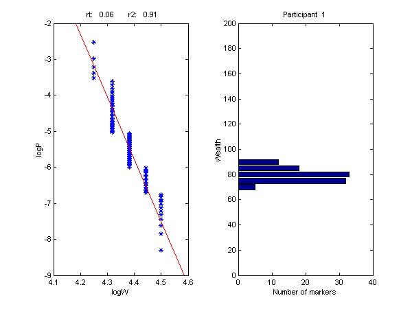
Figure 4 shows the results obtained from the responses of the first participant in the study. The graph on the right shows the distribution chosen by the participant. The graph on the left plots the logarithms of the state prices and the logarithms of the wealth levels assigned to the states in order to achieve the probability distribution at the least cost. The straight line in the left-hand graph plots the relationship obtained by regressing log(w) on log(P). We choose to regress log(w) on log(P) since the respondents are implicitly given state prices and asked to choose wealth levels in various states, so that log(w) is a natural choice for the dependent variable with log(P) the independent variable.
The statistics at the top of the diagram indicate (1) the negative of the slope of this line (rt) and (2) the r-squared value (r2) indicating the extent to which the regression line fits the points.
As the prior discussion showed, the regression line in such a diagram has direct economic meaning in two senses. If a respondent were to choose a distribution that gives points precisely on a line in log(w)/log(P) space then he or she could be characterized as maximizing the expected value of a CRRA utility function. Moreover, in a world in which returns are IID, he or she should follow a constant-mix strategy.
As can be seen, this respondent is relatively conservative, with a risk tolerance of 0.06. This is only one-eighth as large as the risk tolerance for an investor who should hold an all-stock portfolio (0.4668, as shown earlier).
While the points in the diagram for participant 1 do not fall precisely along the line, they fit reasonably well, with differences in state prices explaining 91% of the differences in chosen wealth levels, as shown by the correlation coefficient of 0.91. The mean r2 value for all participants was 0.82. Figure 5 shows the distribution of the r2 values. As can be seen, 25 respondents made choices that were quite close to those of a CRRA investor (r2 greater than 0.90), with another 22 fairly close (r2 between 0.80 and 0.90). On the other hand, 19 of the respondents made choices that differed significantly from those of a CRRA investor. Of these, one chose an all-bond portfolio, with rt=0 and r2=0, which is in fact a constant-mix strategy. For the other 18, however, it could be the case that even in an IID world, a dynamic strategy might be preferable to a constant mix strategy.
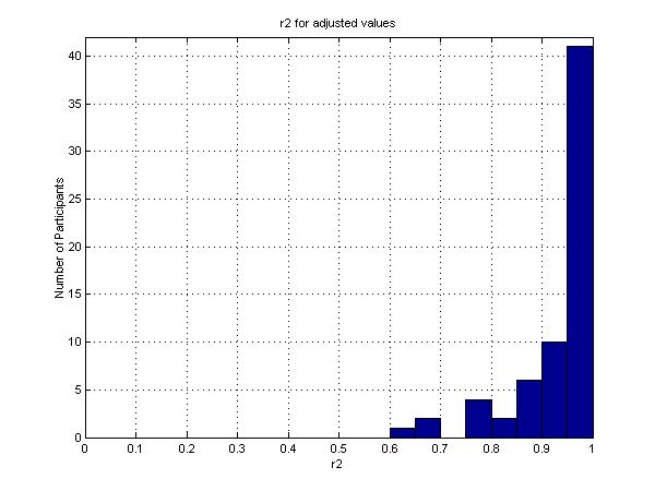
There is reason to believe that these results understate the extent to which the participants' preferences do in fact conform to those of an investor with a CRRA utility function. The survey used a relatively coarse grid, with choices limited to outcomes of 5%, 10%, ..through 200%. Thus a participant who wished to place a marker alongside, say, 68.5% could not do so and presumably would select 70% -- the nearest available row. For this reason, one might choose to consider the r2 value for a participant as a lower bound on the true value. To provide an upper bound, we perform the following adjustment. In each of the 100 states of the world, the chosen amount (e.g. 70) was moved toward the regression line, but no more than 2.5 (half the width of each 5% interval). Figure 6 shows the distribution of r2 values after making these adjustments. In this case, the number of participants with r2 values greater than 0.90 is 51.
Given the limitations of the survey, any conclusions must be tentative at best. The r2 values provide a statistical measure of the appropriateness of a CRRA strategy, not an economic measure, although the two are likely to be correlated. Subject to these caveats, the results are at least suggestive of a conclusion that while constant mix strategies may be acceptable for a majority of investors there could be a meaningfully large minority for whom dynamic strategies may be more desirable.
As noted, the first respondent in the survey adopted a very conservative distribution, with rt = 0.06. The average value of rt for the full set of 66 respondents was 0.12, which is still only slightly more than one-fourth as large as the value for an investor who should choose an all-stock portfolio. For each participant, a constant mix strategy with risk tolerance equal to that of the regression line was determined, to a precision of 0.5%. Figure 7 shows the distribution of the corresponding values for all participants.The mean of the resulting values was 26%5.
All of the participants exhibited risk tolerances below that of an all-stock investor. While this may appear to be inconsistent with practice, it is important to remember that most individuals depend on not only stocks and bonds for their retirement but also a number of lower-risk assets such as rights to social security payments, defined benefit pension plans, short-term savings, real estate and other real assets. Hence the risk tolerances of the participants in the study may not differ significantly from those of other middle-income individuals.
Many portfolio approaches are designed to select combinations of assets that are mean/variance efficient. A portfolio is said to be mean/variance efficient if no other offers (1) the same standard deviation of return and a higher mean return, (2) a smaller standard deviation of return and the same mean return, or (3) a lower standard deviation of return and a higher mean return.
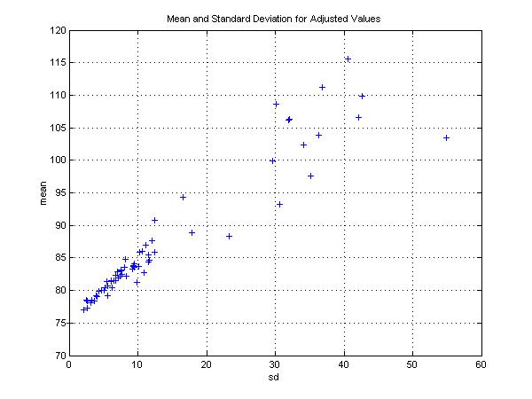
Of necessity, each investment strategy that we consider is mean/variance efficient in the short run (per period or per instant) since there are only two possible investments. However, distributions of chosen ending values need not be mean/variance efficient. The means and standard deviations of the ending values are shown in figure 8 and figure 9, with each participant's distribution represented by a point. Figure 8 uses the distributions as originally chosen, while figure 9 uses the values adjusted to conform more closely to the CRRA approximation..
As the figures show, there is considerable disparity among both the means and in the standard deviations. Moreover, some participants' selections are dominated from a mean/variance perspective, in the sense that another participant's distribution provides a higher mean and lower standard deviation. This is the case even though every distribution is efficient in a least-cost sense, and each provides the maximum feasible expected utility for a utility function that is non-increasing (although not necessarily smooth). This suggests that it may be inappropriate to apply mean/variance optimization to distributions of terminal outcomes obtained after many investment periods. Instead it may be preferable to adopt a constant mix or dynamic strategy utilizing investments that are mean/variance efficient in each investment period.
Thus far we have examined the preferences of individual participants and distributions of the characteristics of those preferences. This is relevant for issues relating to investment counseling, the creation of investment products, and other decisions to made by and for a population of investors with diverse preferences. We turn now to analyses that are more germane for economists and others who construct models of capital market equilibrium. We focus on the second key question. Does the "representative investor" have CRRA preferences? As indicated earlier, models of capital markets that assume IID processes are typically consistent with such preferences. Since we have created a setting in which state prices are generated by such a return process, it is instructive to see if the aggregate of the participants' preferences conforms with those of an investor maximizing the expected utility of a CRRA utility function.
To begin we use a simple characterization of aggregate preferences. Figure 10 shows the number of markers in each wealth row. While the distribution is far from smooth, it appears to be approximately lognormal, as is the distribution of returns from any constant mix in an IID setting. This provides at least suggestive evidence that the aggregate preferences of the participants conform reasonably well to those of an investor with a CRRA utility function.
More precise results can be obtained by aggregating the wealth levels chosen in each of the 100 states. Since we have no evidence on the relative current wealth levels of the participants, we give each the same weight. For ease of interpretation, we then divide the total wealth in each state by the number of participants. The result is a vector of the wealth desired by the representative (here, average) investor in each state. In the remainder of this section all references to wealth refer to that of this representative investor.
Figure 11 plots the logarithms of state prices and wealth levels for the representative investor. The points correspond very well to those on the fitted regression line, which has a risk tolerance of 0.13. The r2 value is 0.98, which is remarkably high, given the coarseness of the survey and the variety of participant choices.
As figure 11 shows, the differences between participants' desired wealth levels and those that could be obtained with a comparable constant mix strategy are relatively small and of little statistical significance. They do exhibit some desire for downside protection but as will be seen, even this is of small economic significance.
The constant mix with the same risk tolerance as that found for the representative investor has 26.5% invested in stocks (to the nearest 0.5%), reflecting the conservatism reflected in the earlier analyses. We thus compare the chosen wealth levels with those obtained from a constant mix strategy with 26.5% invested in stocks. For convenience, we call this a market strategy.
Figure 12 compares the wealth levels for the representative investor (blue curve) and the market strategy (red line). The representative investor chooses to do better than the market strategy in severe bear markets (market strategy <68) and substantial bull markets (market strategy between 95 and 112). In return, the investor falls below the market strategy in modest bear and bull markets (market strategy between 68 and 95) and extreme bull markets (market strategy > 112).
These differences are, however, not very important.
Consider first the issue of market equilibrium. If the survey participants were truly representative, a market with the state prices we have posited would not clear. This would be true even if the market portfolio had 26.5% of its value in stocks and 73.5% in bonds. But equilibrium could easily be attained if another group of investors with equal wealth were willing to suffer more in severe bear markets, do better in moderate markets and extreme bull markets and somewhat worse in substantial bull markets. The curve for such a set of investors would simply be the reflection around the straight line of the representative investor's curve. Moreover, the burden on the other group of investors would not be overly great. For example, even in the worst possible bear market, they would receive a wealth (retirement standard of living) of 55%, while the participant group received 65%. In the best possible bull market they would receive roughly 140%, while the participant group received 115%. It is not implausible that there could be investors with sufficient wealth to provide our more typical investors with insurance against severe bear markets. If so, overall equilibrium could be established.
More important, the economic values of the differences are very small. To illustrate this, we compute the present value of the difference between the wealth of the representative investor and that of the market strategy in each state, then cumulate the resulting values beginning with the state with the lowest market return. For convenience, the cumulative values are expressed as a percent of the participants' initial budget. Figure 13 shows the cumulative sum of these values for each of the outcomes of the market strategy. Figure 14 shows the cumulative sum of the values for each of the 100 states.
Both figures show that the representative investor seeks insurance against severe bear markets but the total value of that insurance is less than 1% of the value of the overall investment. As figure 13 shows, the insurance is paid for primarily by accepting underperformance in states in which the market strategy provides wealth levels between 68 and 95. Interestingly, the values of the differences between the wealth levels for market strategy outcomes over 95 are of very little economic significance.
Figure 14 provides a view of the probabilities associated with the periods of under and over performance. Since each state is equally probable, the horizontal axis can be interpreted as a cumulative probability, with the difference between two points on the horizontal axis representing the probability that the actual state will fall within the range in question. As the figure shows, there is only a 5% probability that there will be a bear market severe enough that the representative investor will outperform the market strategy. On the other hand, there is a 70% probability (75 - 5) that the representative investor will underperform the market strategy. There is approximately a 20% (95 - 75) probability that the representative investor will outperform the market strategy but the value of the outperformance is relatively small. Finally, there is a small probability (less than 5%) that the representative investor will underperform the market strategy, but the economic value of the differences is also extremely small.
Given the small sample size and possible biases in the selection of participants, the results of this survey are, as indicated in the title of the paper, preliminary. Definitive evidence on the issues addressed here awaits more comprehensive surveys. Nonetheless, the results of this survey are at least suggestive of characteristics that might be found when further research is undertaken.
By and large, the choices made by the participants in this survey conform well with the assumption that the representative investor's preferences are close to those of an individual maximizing the expected value of a utility function that exhibits constant relative risk aversion. While there are differences, they are of relatively small significance, both statistically and economically. There is some evidence that the typical participant desires some "downside protection" in severe bear markets, but the markets in question have less than a 5% probability of occurrence and the cost of the desired protection would be less than 1% of the value of the participants' overall positions. With this small exception, these results are broadly consistent with widely-used assumptions about both market return-generating processes and investor preferences.
Even though the aggregate of the participants' desires conforms well to standard assumptions about investor preferences, this was not the case for every individual who participated in the survey. Nonetheless, the majority of participant made choices that did not differ significantly from those made by an investor who maximizes the expected value of a utility function that exhibits constant relative risk aversion, based on a statistical measure of goodness of fit. Due to the coarseness of the set of possible choices, only the range of relevant r-squared values can be estimated, but for between 25 and 51 of the 66 participants the r-squared value for conformance with constant relative risk aversion preferences exceeded 0.90.
These results suggest that a constant mix investment strategy may be appropriate for a majority of investors. However, the presence of a substantial minority with preferences that did not conform well with a constant relative risk aversion utility function suggests that dynamic investment strategies may be preferable for a significant number of investors. More definitive statements require estimates of the expected utility lost if an investor in this minority were to adopt a constant mix strategy and the cost of actually implementing alternative dynamic strategies.
To obtain better evidence on these issues, additional surveys need to be conducted. First and foremost, larger sample sizes need to be obtained. To the extent possible, participants should be representative of a cross-section of investors. Further information should also be obtained. For example, the initial budget could be set randomly, so that one participant could achieve a 75% standard of living without risk, another could achieve 80%, and so on. This would allow tests of hypotheses concerning the effect of wealth on investor preferences. An additional feature might also be invoked after the participant selects a preferred distribution. The participant could be shown a distribution for the constant mix strategy that provides outcomes along the regression line fit to the chosen distribution, then asked to indicate the percent of the initial budget that he or she would be willing to spend to obtain this alternative distribution. The answer would provide a measure of the certainty equivalent value of the alternative distribution and hence a direct economic measure of the expected utility lost by adopting a constant mix strategy.
The results of this preliminary survey suggest that the distribution builder approach can be used to obtain important information about the preferences of individual investors -- information that can prove useful for both those building models of the behavior of capital markets and for those who provide advice to individuals concerning desirable long-term investment strategies. The results obtained here are provocative, but their generality can only be determined with further research.
*. This paper was prepared for presentation at the German Finance Association Meeting in Vienna, Austria on October 5, 2001.
1. William F. Sharpe, Daniel G. Goldstein and Philip W. Blythe, "The Distribution Builder: A Tool for Inferring Investor Preferences," October, 2000, www.wsharpe.com/art/qpaper/qpaper.html
2. This involves relatively few modest assumptions about individual preferences, but it does rule out state-dependent utility and choices in ranges in which the participant's utility might increase at an increasing rate.
3. Note that the stock market has a Sharpe Ratio -- expected excess return divided by standard deviation of excess return -- of 1/3, which is reasonably consistent with both long-term experience and some experimental results concerning individual choice under uncertainty.
4. While some of the relationships we have derived depend on the fact that every state is assumed to be equally probable, it is not difficult to extend the results to cover cases in which states have different probabilities. In such instances the role played here by a state price is placed by the ratio of a state price to its probability. Analysis of a binomial model with different probabilities for the two one-period states will show that the logarithm of the probability of a terminal state will be a linear function of the number of up-branches along the path to that state. Since this is also true of the state prices, there will be a linear relationship between the logarithm of the ratios of the state prices to probabilities and the number of up-branches. Since a similar relationship holds for the values of terminal wealth for any constant mix strategy, the qualitative results that we have obtained thus far will hold, even in this broader setting.
5. There was no relationship between the r2 and rt values -- the r-squared value for a regression of the former on the latter was only 0.02.
Figure 1: Playing Field Rows
Figure 2: Controls and The Budget Indicator
Figure 3: Questions Concerning Participant Experience
Have you completed this survey before?
No
YesHow would you describe this session?
I was just playing around
I spent some time but not enough to take my choice seriously
This may represent my choice but I could probably improve on it
This is probably pretty close to the best for me
This is almost certainly the best for me
Figure 4: Participant 1 Data
Figure 5: R2 Distribution for Original Values
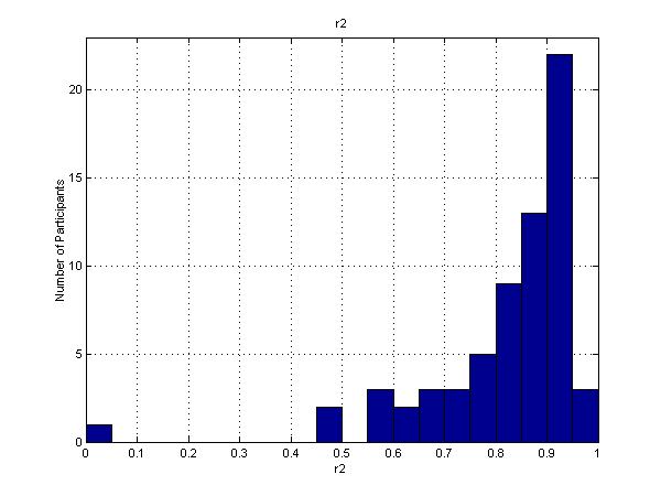
Figure 6: R2 Distribution for Adjusted Values
Figure 7: Distribution of Constant Mix Strategies
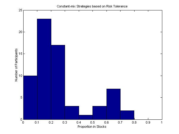
Figure 8: Means and Standard Deviations for Original Values
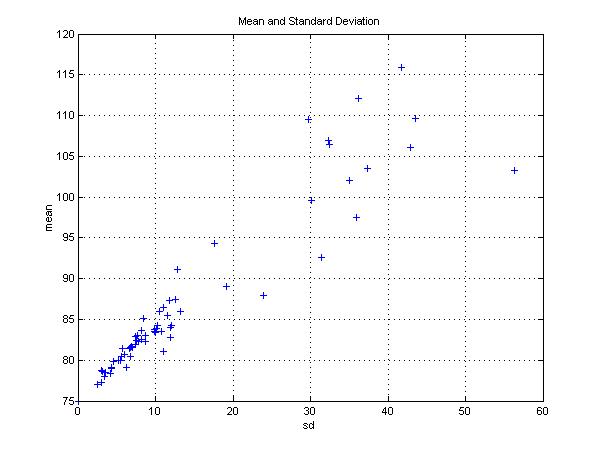
Figure 9: Means and Standard Deviations for Adjusted Values
Figure 10: Distribution of Aggregate of All Markers
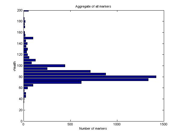
Figure 11: Desired Aggregate Wealth Levels and State Prices
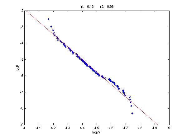
Figure 12: Wealth Levels for the Representative Investor and a Market Strategy
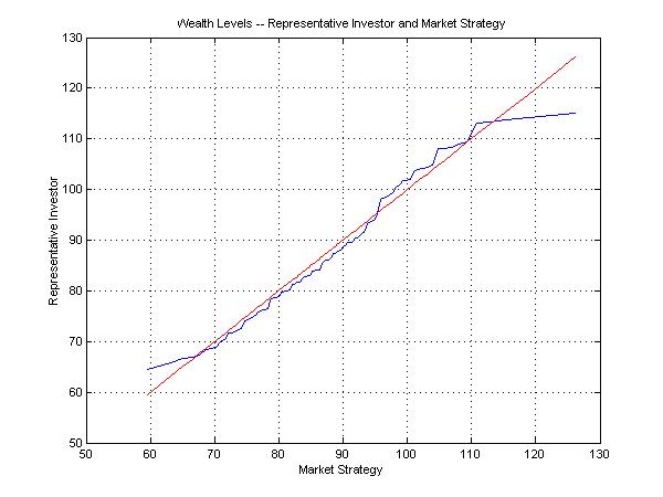
Figure 13: Cumulative Value of Differences and Market Strategy Outcomes
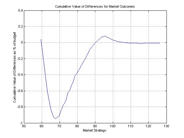
Figure 14: Cumulative Value of Differences and States
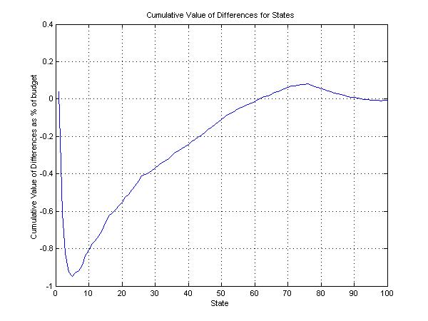
Table 1: Respondents and Time Spent by Category
Description |
Number of Respondents | Average Time spent (minutes) |
| I was just playing around | 0 | -- |
| I spent some time but not enough to take my choice seriously | 1 | 17.7 |
| This may represent my choice but I could probably improve on it | 34 | 17.0 |
| This is probably pretty close to the best for me | 28 | 20.0 |
| This is almost certainly the best for me | 3 | 14.7 |
| All Respondents | 66 | 18.2 |