
The world is, unhappily, very complex. Before one can analyze, one must abstract. The time-state paradigm provides a procedure for doing so. Its power lies in the straightforward way that it accommodates time, risk, and options. But this power comes at a price. In general, one must assume a relatively simple structure (e.g. two possible outcomes in each trading period) and the existence of markets that are sufficiently complete to allow replication and valuation of desired patterns of payments and/or consumption over time.
Despite these limitations, the time-state paradigm is eminently practical in a number of settings. Dynamic strategies involving broad asset classes are frequently analyzed using it. It is also the paradigm of choice when derivative securities are the focus of attention. However, when the goal is to consider many possible combinations of many different financial instruments, use of the time-state approach poses a number of problems. One must either assume a limited number of outcomes in each trading interval, making most of the securities redundant, or many such outcomes, making the assumption of complete markets unrealistic. Clearly, a Hobson's choice.
In 1952, Markowitz proposed a paradigm for dealing with issues concerning choices which involve many possible financial instruments. Formally, it deals with only two discrete time periods (e.g. "now" and "a year from now"), or, equivalently, one accounting period (e.g. "one year"). In this scheme, the goal of an Investor is to select the portfolio of securities that will provide the best distribution of future consumption, given his or her investment budget. Two measures of the prospects provided by such a portfolio are assumed to be sufficient for evaluating its desirability: the expected or mean value at the end of the accounting period and the standard deviation or its square, the variance, of that value. If the initial investment budget is positive, there will be a one-to-one relationship between these end-of-period measures and comparable measures relating to the percentage change in value, or return over the period. Thus Markowitz' approach is often framed in terms of the expected return of a portfolio and its standard deviation of return, with the latter serving as a measure of risk.
The Markowitz paradigm is often characterized as dealing with portfolio risk and (expected) return or, more simply, risk and return. More precisely, it can be termed the mean-variance paradigm.
Assume that a portfolio will have a future (end-of-period) value of v1 in state 1, v2 in state 2, etc.. let v = [v1,v2,...vm] be a {1*m} element vector, where m is the number of possible states of the world. To compute the portfolio's expected future value, we need someone's estimate of the probabilities associated with the states. Let pr = [pr1,pr2,...,prm] be such a vector. The expected value is, as usual, a weighted average of the possible outcomes, with the probabilities of the outcomes used as weights:
ev = pr*v'
If the current value of the portfolio is p, we can compute a vector of value-relatives (future/present values):
vr = v/p
And a vector of returns (proportional changes in value):
r = (v-p)/p
The portfolio's expected value-relative can be computed either directly or indirectly:
evr = (pr*v')/p = ev/p
Similarly, the portfolio's expected return will be:
er = (pr*(v-p)')/p = ((pr*v')-p)/p = (ev-p)/p
In the special case in which every outcome is equally likely, the expected value can be computed by simply taking the (arithmetic) mean of the possible values. In MATLAB:
ev = mean(v)
Note that the mean function can be used with a matrix -- the result will be a row vector in which each element is the mean of the corresponding column in the original. This can prove handy with a matrix in which each column represents a different asset and each row a different state of the world, with the latter assumed to be equally likely.
Probability estimates are essential in the mean-variance approach. Unless all Investors agree about such probabilities, one cannot talk about "the" expected value or expected return (or risk, for that matter) of a portfolio, security, asset class or investment plan. Two different Analysts might well provide different estimates of expected values for the same investment product. Indeed, one of the key functions than an Analyst can perform for an Investor is the provision of informed estimates of the probabilities of various outcomes and the associated risks and expected values of alternative investment strategies.
Normative applications of the mean-variance paradigm often accept the possibility of disagreement among Investors and Analysts concerning probability estimates. Positive applications usually assume either that there is agreement concerning such probabilities or that prices are set as if there were agreement on a set of consensus probability estimates.
It is important to emphasize the fact that the mean-variance approach calls for the use of estimates of the probabilities of alternative future possible events in the next period. Historic frequencies of such events in past periods may prove helpful when forming such forward-looking estimates, but one should consider taking into account any additional information that might prove helpful. The world changes, and the future need not be like the past, even probabilistically. Issues concerning ways to implement the mean-variance approach can and should be separated from issues concerning its structure, assumptions, and implications.
If the future value of a portfolio will be vs in state s and the expected future value is ev, the deviation, or surprise, in state s will equal (vs-ev). More generally, if v is the vector of possible future values, the vector of deviations, state by state, will be:
d = v - ev
In this vector, a positive deviation represents a happy surprise, a negative deviation an unhappy surprise, and a zero deviation no surprise at all. Roughly: the greater the "spread" of the possible deviations, the greater the uncertainty about the actual outcome.
To measure risk in a fully useful manner we need to take into account not only the possible surprises, but also the probabilities associated with them. Simply weighting each deviation by its probability won't do, since the answer will always equal zero.
One alternative uses the expected or mean absolute deviation (mad):
mad = pr*abs(d)'
In practice, it is difficult to use mad measures when considering combinations of securities and portfolios. Mean-variance theory thus utilizes the expected squared deviation, known as the variance:
var = pr*(d.^2)'
Variance is often the preferred measure for calculation, but for communication (e.g between an Analyst and an Investor), variance is usually inferior to its square root, the standard deviation:
sd = sqrt(var) = sqrt(pr*(d.^2)')
Standard deviation is measured in the same units as the original outcomes (e.g. future values or returns), while variance is measured in such units squared (e.g. values squared or returns squared).
We again emphasize that standard deviation is used in this context as a forward-looking measure of risk, since it is based on probabilities of future outcomes, however derived. One can assume that future risk is similar to past variability, but this is neither required nor, in certain cases, desirable.
MATLAB provides a function for computing the standard deviation of a series of values, and one that can be used to compute the variance of such values. In each case, the computations assume that the outcomes are equally probable. In addition, it is assumed that the values are drawn from a sample distribution taken from a larger population., and that the variance and standard deviation of the population are to be estimated.
For reasons that we will not cover here, the best estimate of the population variance will equal the sample variance times n/(n-1), where n is the number of sample values. Correspondingly, the best estimate of the population standard deviation will equal the sample standard deviation times the square root of n/(n-1). MATLAB'a functions make this correction automatically, as do many functions included with spreadsheet software. When estimates of this type are desired, one can use std(v) to find the estimated population standard deviation where v is a vector of sample values. Alternatively, one can use cov(v) to find the estimated population variance. Note that both functions are inherently designed to process historic data in order to make predictions about future results and hence implicitly assume that future "samples" will be drawn from the same "population" as were prior ones. In some cases this assumption may be entirely justified; in others it may not.
Thus far, we have dealt with a world in which a future value can take on one of a discrete set of specified values, with a probability associated with each value. The mean-variance approach can be utilized in such a setting, and we will do this from time to time for expository purposes. However, its natural setting is in a world in which outcomes can lie at any point along a continuum of values. Statisticians use the term random variable to denote a variable that can take on any of a number of such values.
In a discrete setting, the actual value of a variable will be drawn from a vector (e.g. v) having a finite number of possible outcomes, with the probability of drawing each value given by the corresponding entry in an associated probability vector (e.g. pr). The set of values (v) and the associated probabilities (pr) constitute a discrete probability distribution.
In a continuous setting, a value will be drawn from a continuous probability distribution, the parameters and form of which indicate the range of outcomes and the associated probabilities.
The most informative way to portray a distribution utilizes a plot of the probability that the actual outcome will be less than or equal to each of a set of possible values.
Let v be a vector of values, sorted in ascending order, and pr a vector of the probabilities associated with each of the corresponding values. For example:
v = [ 10 20 30];
pr = [ 0.20 0.30 0.50];
The probability that the actual outcome will be less than or equal to 10 is 0.20. The probability that the actual outcome will be less than or equal to 20 is (0.20+0.30), or 0.50, and the probability that the outcome will be less than or equal to 30 is 1.00. To produce a vector of these probabilities we can use the MATLAB cumsum function, which creates a new vector in which each element is the cumulative sum of all the elements up to and including the comparable position in the original vector. In this case:
cumsum(pr) =
0.2000 0.5000 1.0000
The figure below shows the associated cumulative probability distribution. Note that it is a step function, reflecting the discrete nature of the outcomes.
It is, of course, much simpler to simply plot the points, and let MATLAB connect them with straight lines. Here are the required statements:
plot(v,cumsum(pr));
xlabel('outcome');
ylabel('Probability actual <= outcome');
In this case the result is:

The greater the number of points and the nearer together they are, the closer will be this type of plot to the more accurate step function. In the case of a continuous distribution, there will be no difference at all.
A uniformly-distributed random variable can take on any value within a specified range (e.g., zero to one) with equal probability. Most programming languages and spreadsheets provide functions that can generate close approximations to such variables (purists would, however, call them pseudo-random variables, since they are not completely random). In MATLAB, the function rand(r,c) generates an {r*c} element matrix of such numbers.
Consider the process of generating 1000 sets of 1000 such numbers, then taking the mean (unweighted average) of each set. In MATLAB:
z = mean(rand(1000,1000))
A histogram showing the frequency distribution of the mean values in each of 25 "bins" can be obtained with the statement:
hist(z,25)
The figure below shows the results obtained in this manner in one experiment.

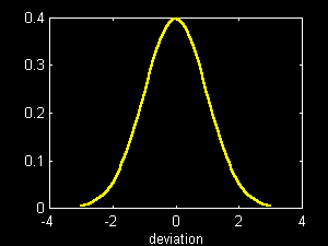
Note that the distribution is approximately "bell-shaped" and roughly symmetric. This is not surprising since the central limit theorem holds that the distribution of the sum or average of a set of unrelated variables will approach a particular form as the number of variables increases. The form is that of the normal distribution, given by the equations:
nd = (x - ev)/sd;
p(x) = (1/sqrt(2*pi))*exp(-(nd^2)/2)
where p(x) is proportional to the probability that the actual value will equal x; ev and sd stand for the expected value and standard deviation, respectively, of the distribution, and nd is the deviation of x from ev in standard deviation units.
The figure below plots p(x) for various values of nd.
More practical is the cumulative normal distribution . MATLAB does not provide such a function, but it offers the next best thing. The expression erf(x)/sqrt(2)) gives the probability that a normally-distributed random variable will fall between -x and +x standard deviations of the mean. This forms the basis for our function cnd(nd) where nd is a standardized deviation and cnd(nd) is the probability that the actual outcome will be less than nd.
The figure below shows the values of cnd(nd) for nd from -3 to +3 (in steps of 0.1), using the MATLAB statements:
nd = -3:0.1:3;
pr = cnd(nd)
plot(nd,pr);
grid;
xlabel('deviation');
ylabel('Probability actual <= outcome');
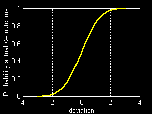
The cumulative normal distribution can be used to determine probabilities that a normally-distributed outcome will lie within a given range. For example, the probability that an outcome will like within one standard deviation of the mean is:
cnd(1)-cnd(-1)
0.6827
Thus there are roughly two chances out of three that the outcome will lie within this range. Some characterize an investment's prospects by giving its mean and standard deviation in the form: e +/- sd (read as e plus or minus sd); thus an asset mix might be said to offer returns of 10+/-15. If the return can be assumed to be normally-distributed, this means that there are roughly two chances out of three that the actual return will lie between -5% (10-15) and 25% (10+25).
The probability that a normally-distributed return will be within two standard deviations of the mean is given by:
cnd(2)-cnd(-2)
0.9545
Thus if a normally-distributed investment is characterized by 10+/-15, the chances are roughly 95% that its actual return will lie between -20% (10 - 2*15) and 40% (10+2*15).
In MATLAB one can produce normally-distributed random variables with an expected value of zero and a standard deviation of 1.0 directly using the function randn. Thus:
z = ev + randn(100,10)*sd
will produce a {100*10} matrix z of random numbers from a distribution with a mean of ev and a standard deviation of sd.
While the central limit theorem provides a powerful inducement to assume that investment returns and values are normally distributed, it is not sufficient in its own right. While most investment results depend on many events and most portfolios contain many securities, it is unlikely that the influences on overall results are unrelated. If, for example, the health of an economy is not normally distributed, and if it affects most securities to at least some extent, even the value of a diversified portfolio will have a non-normal distribution.
To solve this problem at a formal level, Analysts often assume that the return or value of every investment is normally distributed as is the value or return of any possible combination of investments. Since knowledge of the expected value and standard deviation of a normal distribution is sufficient to calculate the probability of every possible outcome, this very convenient assumption implies that the expected value and standard deviation are sufficient statistics for investment choices in which an end-of-period value or return is the sole source of an Investor's utility.
If the value or return of every possible investment and combination of investments is normally distributed, we say that the set of such variables is jointly normally distributed .The mean-variance approach is well suited for application in such an environment.
Some argue that standard deviation is a flawed measure of risk since it takes into account both happy and unhappy surprises, while most people associate the concept of risk with only the latter. Alternative measures focus on "downside risk" or likely "shortfall". Each requires the specification of an additional parameter -- the point from which shortfall is to be measured. This threshold may be zero, a riskless rate of return, or some level below which the Investor's disappointment with the outcome is assumed to be especially great.
The simplest shortfall measure is the probability of a shortfall below a stated threshold. This can be read directly from a graph of the associated cumulative distribution. For example, assume that the probability that a return will be less than 10% is desired. In the figure below, find 10% on the horizontal axis. Go up to the curve, then over to the vertical axis. The result is 0.5. Thus there is a 50% probability that the return will fall below the selected threshold of 10%.

More complex shortfall measures take into account all possible outcomes below the selected threshold and their probabilities to obtain an estimate of the "likely" magnitude of the shortfall. Let r be a vector of possible returns and pr a vector of the associated probabilities. For example:
r = [-10 0 10 20]
pr = [.1 .2 .3 .4]
Assume that the desired threshold is 10 (%). The positions in r which contain returns below the threshold can be found simply using the MATLAB expression:
r<threshold
1 1 0 0
To produce a vector of shortfalls we subtract the threshold from each return, then multiply the resulting vector by the vector that contains zeros in all positions in which the difference is positive:
sf = (r-threshold).*(r<threshold)
-20 -10 0 0
To find the expected shortfall multiply each of these values times the associated probability:
pr*sf'
-4
An alternative is the semi-variance, which is the expected squared shortfall:
pr*(sf.^2)'
60
The square root of the semi-variance is termed the semi-standard deviation. In a sense, it is the "downside" counterpart of the standard deviation. In the case at hand:
sqrt(pr*(sf.^2)')
7.7460
The expected shortfall, the semi-variance and the semi-standard deviation are all unconditional measures. For example, the expected shortfall is the expected value of the shortfall, whether there is one or not. All outcomes that exceed the threshold are treated equally (as zero shortfalls), no matter what their magnitude. Alternative measures answer a somewhat different set of questions. For example, one might wish to know the size of the expected shortfall if there is one. More directly: conditional on the existence of a shortfall, how large is it likely to be?
To compute a conditional measure, only states of the world in which a shortfall occurs are considered. The desired probabilities are those conditional on such a situation arising. In our example, only the first two states of the world produce shortfalls. The associated unconditional probabilities are 0.1 and 0.2. Thus the probability of a shortfall is 0.3. The conditional probabilities for the two states are 0.3333 (=0.1/0.3) and 0.6667 (=0.2/0.3).More generally, we divide each unconditional probability by the probability of a shortfall. To find the latter we need a vector of the unconditional probabilities for states in which there is a shortfall:
pr.*(r<threshold)
0.1000 0.2000 0 0
The sum of these values is the probability of a shortfall:
prsf = sum(pr.*(r<threshold))
0.3000
To find the conditional expected shortfall, we could divide each unconditional probability by this value, then multiply by the shortfall vector. Equivalently, we could simply divide the unconditional expected shortfall by the probability of a shortfall:
pr*sf'/prsf
-13.3333
Earlier we found that the expected shortfall is 4%. However, if there is a shortfall, the expected amount is 13.33%.
Similarly, the conditional semi-variance equals the unconditional semi-variance divided by the probability of a shortfall. From this it follows that the conditional semi-standard deviation equals the unconditional semi-standard deviation divided by the square root of the probability of a shortfall.
Another measure of downside risk is based on a specified probability. In effect one asks the question: what is the (almost) worst thing that can happen? A probability px is selected. The associated (almost) worst thing that can happen is given by a return or future value x, such that there is only a 1% probability that the actual outcome will be worse than x.
Assume, for example, that a bad outcome is specified as one that will not be underperformed more than 10% (px) of the time. In the case shown in the previous figure, this is easily determined. Locate 0.1 (10%) on the vertical axis. Then go over to the curve and down to the horizontal axis. The result is -10%. Thus the (10%) worst case involves a return of -10%.
When the result of this kind of calculation involves a negative change in value, the change is often termed the value at risk. Thus, in our example, if the current amount invested were $500,000, we would say that the value at risk is $50,000.
Value at risk is often calculated for short holding periods (e.g. a day or a week). In such cases the expected return is often assumed to be zero. This allows the Analyst to concentrate on the shape of the distribution of returns and its standard deviation, thereby lending at least a somewhat greater sense of objectivity to the result.
In many cases it proves helpful to summarize the prospects of an investment strategy in terms of (1) its expected outcome and (2) a measure of downside risk or likely shortfall, even though the analysis leading to its choice utilized standard deviation as a measure of risk.
Among strategies with equal expected outcomes there is often a one-to-one correspondence between standard deviation and each of several alternative risk measures, including downside ones. Since calculations are far easier when standard deviation is utilized, we follow common practice by utilizing it in much of what follows. When issues of communication are paramount, however, we will include transformations to alternative measures that focus attention on bad outcomes rather than all outcomes.