Marginal Risk	Implied EER
Cash Manager	0	0
Bond Manager	150	2
Stock Manager	450	6

Not surprisingly, the implied values of the asset EER's are identical to those that were used in the optimization process.

Computing Proportions of Dollar Expected Excess Return

Given expected excess returns, we can compute dollar expected excess returns as before as well as the proportions of total dollar expected excess return.  However, the latter will be the same regardless of risk tolerance, and can be computed solely from the covariance matrix and portfolio composition.  Defining P$EER_i as the proportion of dollar expected excess return provided by manager i:

          P$EER_i =  X_i EER_i  /  S_i ( X_i EER_i )

                      =    ( X_i MR_i / rt ) /  S_i ( X_i MR_i / rt )

                      =    X_i MR_i /  S_i ( X_i MR_i )

This relationship both explains and justifies the computations that lie behind mean/variance risk budgeting and management. Marginal risks act as surrogates for expected excess returns.  An overall fund should be managed so that the marginal risk of each of its components is commensurate with the expected excess return of that component. Given expectations about returns, a risk budget can be established, with each component allowed to have a marginal risk (MR_i) and fund allocation (X_i) that give it an appropriate contribution (P$EER_i).

Portfolio Risk Decomposition

Recall from our earlier discussion that the marginal risk of a portfolio component will equal twice its covariance with the portfolio.  From the properties of covariance we know that:

         S_i X_i MR_i  = S_i X_i 2 C_ip = 2 S_i XC_ip = 2 V_p

Thus the sum of the weighted marginal risks of the portfolio components will equal twice the variance of the overall portfolio. This leads some to define the risk contribution of a component as half its marginal risk (that is, its covariance with the portfolio) so that a weighted average of these values will equal the variance of the overall portfolio.  Clearly, this will have no effect on the P$EER_i values.  However, it sometimes leads to an incorrect view that it is possible to decompose portfolio risk into a set of additive components and to incorrect statements of the form "this manager contributed 15% to the total risk of the portfolio".

There is a case in which computations based on marginal risks do provide an additive decomposition of total portfolio risk. If all component returns are independent, the marginal risk of manager i will equal 2X_iV_i and the product X_iMR_i will equal 2X_i²V_i.  Summing these values over managers will give an amount equal to twice the portfolio variance. In this special case, defining a manager's risk contribution as half its marginal risk thus makes the product X_iMR_i equal precisely its contribution to total portfolio risk.

We will see that the assumption of independence may be appropriate for the portion of a manager's return that is not related to the factors included in the underlying factor model and that this interpretation of risk decomposition can be applied to that portion of overall portfolio variance.  Much of the literature on risk budgeting and monitoring focuses on such non-factor risk and thus is justified in claiming that the procedures provide an allocation of portfolio risk.  However, this is not applicable for the correlated components of a pension fund, which generate most of its risk.

Humans best process information when relationships are linear.  Expected returns are linear, and the expected return of a portfolio can be decomposed into portions provided by each of the portfolio components.  This is not generally the case for risk.  For this reason, the computations we have described, which are utilized in many pension fund mean/variance risk budgeting and monitoring systems are best viewed in terms of implied expected excess return budgets and deviations therefrom.

Pension Fund Risk Budgeting and Monitoring in Practice

In practice pension fund risk budgeting and monitoring involves three related but somewhat separate phases. 

In the first phase, the fund selects a policy portfolio in which dollar amounts are allocated to managers.  As indicated earlier, this often involves two stages: (1) an asset allocation or asset/liability study using optimization analysis that allocates funds among asset classes, and (2) the subsequent allocation of funds among managers using procedures which may be quantitative, qualitative or a combination of both. Rarely is the policy portfolio determined entirely by mean/variance optimization, and even the optimization analysis utilized as part of the process often involves binding constraints so that the first order conditions we have described will not hold strictly for every component. In any event, we term this entire process the policy phase. Part of the process will use expected returns and covariances, which we term the policy expected returns and policy risks and correlations. It will also use a (possibly implicit) factor model which we will term the policy factor model. The output of this phase is the policy portfolio, which allocates specific amounts of capital to each of the components of the fund.

The second phase is the establishment of the fund's risk budget. This makes the (possibly heroic) assumption that the policy portfolio is optimal in a mean/variance sense at the time of its designation.  Ideally this would be interpreted using the policy factor model and policy expected returns and covariances.  However, the very nature of the policy phase may make this impossible, since there are typically insufficient estimates of risks and returns, and in most cases the policy portfolio is not created directly from a formal unconstrained optimization.  In practice, therefore, a more complete factor model and set of risks and correlations, typically provided by an outside vendor, is used to perform a reverse optimization based on the policy portfolio as of the date of its formation.  This yields a series of implied expected excess returns and proportions of the portfolio's dollar expected excess return attributable to each component.  Such values represents the components' risk budgets (RB).  From our previous formulas this can be stated most directly as:

RB_i = X_iC_ip / V_p

for each manager i.

Even if the policy portfolio is implemented precisely when the policy phase is completed, market movements, manager actions and changing risks and correlations will lead to changes in many or all aspects of the situation. This leads to the third phase.  Current estimates of risks and correlations, typically provided by the outside vendor, along with manager positions and/or return histories, are used to compute a new set of values for investment proportions, covariances and portfolio variance. This provides the current set of  risk proportions (RP).  Letting primes denote current values, we have:

RP_i = X_i'C_ip' / V_p'

The monitoring phase involves comparisons of the current risk proportions with the risk budgets. Significant disparities lead to evaluation, analysis and in some cases action.

Not surprisingly, this process can easily be misunderstood and misused. The risk budget figures are actually surrogates for proportions of expected value added (over cash) at the time of the policy analysis.  The risk proportion figures are surrogates for the proportions of implied expected value added, based on the current situation.  The presumption is that large disparities need to be justified by changes in estimates of the abilities of the manager to add value. Lacking this, some sort of action should be taken.   Note, however, that a change in a manager's RP value may be due to events beyond his or her control. Moreover, there are many ways to change a manager's RP value if such a change is needed.  The amount invested (X_i) may be adjusted, as may the covariance of the manager's retrun with that of the portfolio.  The covariance may, in turn, be changed by altering the manager's investment strategy or by changing the allocation of funds among other managers and/or the strategies of other managers.

In any event, the comparison of RP values with RB values provides a discipline for monitoring an overall portfolio to insure that it remains reasonably consistent with original or modified estimates of the abilities of the managers. While the actions to be taken in the event of significant disparities are not immediately obvious, it is important to know when actions of some sort are desirable

The diagram below shows the three phases.

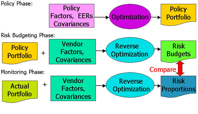
The policy phase is performed periodically, followed by the risk budgeting phase. The monitoring phase is then performed frequently, until the process begins anew with another policy phase.

Incorporating Liabilities

Thus far we have ignored the presence of liabilities, assuming that all three phrases focus on the risk and return of the fund's assets.  However, this may not be appropriate for a fund designed to discharge liabilities. Fortunately, the procedures we have described can be adapted to take liabilities into account.

We continue to utilize a one-period analysis. Current asset and liability values are A₀ and L₀, respectively.  At the end of the period the values will be A₁ and L₁, neither of which is known with certainty at present. We define the fund's surplus as assets minus liabilities.  Thus S₀=A₀-L₀ and S₁=A₁-L₁. We assume that the fund is concerned with the risk and return of its future surplus, expressed as a portion of current assets, that is S₁/A₀.  Equivalently,

S₁ / A₀ = (A₁/ A₀ ) - ( L₀ / A₀ ) * ( L₁ / L₀ )

The first parenthesized expression equals 1 plus the return on assets, while the last parenthesized expression can be interpreted as 1 plus the return on liabilities.   Defining the current ratio of liabilities to assets (L₀/A₀) as the fund's debt ratio (d), S₁/A₀ may be written as:

(1-d) + R_A - d*R_L

The parenthesized expression is a constant and hence cannot be affected by the fund's investment policy.  We thus consider only the difference between the asset return ( R_A ) and the liability return multiplied by the debt ratio (d*R_L ).

We are now ready to write the expected utility as a function of the expected value and risk of  ( R_A - d*R_L )Let rt be the fund's risk tolerance for surplus risk.  Then:

EU = E( R_A ) - E( d* R_L ) - V( R_A - d*R_L ) / rt

Expanding the variance term gives:

EU = E( R_A ) - E( d* R_L ) - V( R_A ) / rt + 2*d*C_AL / rt - d²*V_L  / rt

Since the decision variables are the asset investments, we can ignore terms that are not affected by them.  Neither the expected liability return nor the variance of the liability return is affected by investment decisions.  Hence for optimization and reverse optimization purposes we can define expected utility as:

EU = E( R_A ) -  V( R_A ) / rt + 2*d*C_AL / rt

Note that this differs from expected utility in the case of an asset-only optimization only by the addition of the final term, which includes the covariance of the asset return with the liabilities.  Moreover, covariances are additive, so that the covariance of the asset portfolio with the liabilities will equal a value-weighted average of the covariances of the components with the liabilities. This implies that the marginal expected utility of component i will equal:

MEU_i = EER_i - MR_i / rt  +  2*d*C_iL   /rt

where  C_iL  is the covariance of the return of asset i with that of the liabilities.

We can now write the first order condition for optimality in an asset/liability analysis as:

MEU_i = EER_i - MR_i / rt  +  2*d*C_iL / rt  = k   for each asset i

But the risk-free asset (here, cash) has zero values for all three components.   Hence, as before, k=0 so that:

EER_i - MR_i / rt  +  2*d*C_iL / rt  = 0

and:

EER_i  =  MR_i / rt  -  2*d*C_iL / rt  

To compute implied expected excess returns we need only subtract the covariance of an asset with the liability from its marginal risk, then divide by risk tolerance.   Alternatively, recalling that MR_i= 2*C_ip , we can write:

EER_i  =  (2 / rt ) * ( C_ip - d*C_iL )

All the procedures described in the asset/only case can be adapted in straightforward ways to incorporate liabilities. For example, the risk budgets and risk positions can be determined using the following formulas:

RB_i = [ X_i * ( C_ip - d*C_iL ) ]    /    [ V_p - d*C_pL ]

RP_i = [ X_i' * ( C_ip' - d'*C_iL' ) ] /  [ V_p' - d'*C_pL' ]

where, as before, the variables without primes reflect values at the time of the policy analysis and the variables with primes reflect values at the current time. Due to the properties of variances and covariances, the values of RB_i will sum to one, as will the values of RP_i.

Factor Models

As indicated earlier, most risk estimation procedures employ a factor model to provide more robust predictions. Generically, such a model has the form:

R_i = b_i1F₁ + b_i2F₂ + .... + b_inF_n + e_i

where b_i1, b_i2, ...., b_in  are the sensitivities of R_i to factors F₁, F₂, ...,F_n , respectively and e_i is component i's residual return. Each e_i is assumed to be independent of each of the factors and of each of the other residual returns.

A risk model of this type requires estimates of the risks (standard deviations) of each of the factors and of each of the residual returns.  It also requires estimates of the correlations of the factors with one another.

Note that in this model each return is a linear function of the factors.  We may thus aggregate, using the proportions held in the components to obtain the portfolio's return:

R_p = b_p1F₁ + b_p2F₂ + .... + b_pnF_n + e_p

where each value of b_p is the value-weighted average of the corresponding b_i values and e_p is the value-weighted average of the e_i values.

It is convenient to break each return into a factor-related component and a residual component. Defining R_Fi  as the sum of the first n terms on the right-hand side of the equation for R_i, we can write:

R_i = R_Fi + e_i

Similarly, for the portfolio:

R_p = R_Fp + e_p

Now consider the covariance of component i with the portfolio.  By the properties of covariance, it will equal

C_ip = cov( R_Fi + e_{i ,} R_Fp + e_p ) = cov( R_Fi , R_Fp ) + cov ( R_Fi , e_p )    +  cov( e_i , R_Fp )   + cov( e_i ,  e_p  )

By the assumptions of the factor model, the second and third covariances are zero.   Hence:

C_ip =  cov( R_Fi , R_Fp )  + cov( e_i ,  e_p  )

Recall that:

          e_p =  S_i  X_i e_i 

Since the residual returns are assumed to be uncorrelated with one another, the covariance of e_i with e_p is due to only one term. Let v_i be the variance of e_i (that is, component i's residual variance).   Then:

cov( e_i ,  e_p  ) = X_i v_i

and

C_ip =  cov( R_Fi , R_Fp )  + X_i v_i

Substituting this expression in the formula for the implied excess return in the presence of liabilities we have:

EER_i  =  (2 / rt ) * (  cov( R_Fi , R_Fp )  + X_iv_i - d*C_iL )

This can be regrouped into two parts -- one that would be applicable were there no residual risk, and one that results from such risk:

EER_i  =  (2 / rt ) * [ cov( R_Fi , R_Fp )   - d*C_iL ]  + (2 / rt )*X_iv_i

The final term is often termed the manager's alpha value -- that is the difference between overall expected return and that due to the manager's exposures to the factors (and here, covariance with the fund's liability). Thus we have:

EER_i  =  Factor-related EER_i  +  a_i

where:

Factor-related EER_i  = (2 / rt ) * (  cov( R_Fi , R_Fp ) - d*C_iL )

and

a_i  = (2 / rt ) *  X_iv_i

Just as implied expected returns can be decomposed into factor-related and residual components, so too can risk budgets and risk proportions. For example, a manager could be given a budget for factor-related contributions to risk and a separate budget for residual risk.  Many systems concentrate on the latter, which has substantial advantages since, as indicated earlier, the contributions to portfolio residual risk do in fact add to give the total portfolio residual variance. However, they cover only a small part of the total risk of a typical pension fund.

Aggregation

Expected excess returns are additive.  Thus the expected excess return for a group of managers will equal a weighted average of their expected excess returns, using the relative values invested as weights.  Covariances are also additive.  Thus the marginal risk of a group of managers can be computed by weighting their marginal risks by relative values invested.  This makes it possible to aggregate risk budgets and risk proportions in any desired manner.  For example, a fund may be organized in levels, with each level's risk budget allocated to managers or securities in the level below it, and so on. Thus there could be a risk budget for equities, with sub-budgets for domestic equities and international equities.  Within each of these budgets there may be sub-budgets for individual managers, and so on.

An Example

The following tables provide an example for a large pension fund.  These results were obtained using an asset-class factor model with historic risk and correlation estimates. The relationships of the managers to the factors were found using returns-based style analysis. Residual variances are based on out-of-sample deviations from benchmarks based on previous returns-based style analyses. After the managers were analyzed, they were combined into groups based on the fund's standard classifications. Implied expected excess returns were calibrated so that a passive domestic equity portfolio would have the expected excess return used in thef und's  most recent asset allocation study. Although the fund does take liabilities into account when choosing its asset allocation, the figures shown here are based solely on asset risks and correlations.

                                                        Implied Expected Excess Returns (EER)

	Factor-related	Alpha	Total
Cash Equivalents	0.02	0.00	0.02
Fixed Income	1.53	0.00	1.53
Real Estate	4.01	0.36	4.36
Domestic Equity	5.66	0.03	5.69
International Equity	4.82	0.03	4.84
Int'l Fixed Income	1.42	0.00	1.42
Global Asset Allocation	3.79	0.00	3.79
Special Assets	3.13	0.26	3.40

Note that the implied alpha values are all small, including four that are less than 1/2 of 1 basis point and thus shown as 0.00.  This is not unusual for funds with many managers. A high degree of diversification is consistent with relatively low expectations concerning managers' abilities to add value.

As we have shown, the implied expected excess returns can be combined with the amounts allocated to the managers to determine the implied expected values added over a cash investment, which we have termed the dollar expected excess returns ($EER).  These can be divided by the total $EER for the portfolio to show the relative contribution to excess expected return for each manager or aggregate thereof.  The final three columns of the following table shows the results for the fund in question, broken into the factor-related component and residual-related component (alpha).

                                            Percents of Implied Portfolio Dollar Expected Excess Return

	% of $	% of $EER: Factor-related	% of $EER: Alpha	% of $EER: Total
Cash Equivalents	1.72	0.01	0.00	0.01
Fixed Income	21.30	7.69	0.02	7.71
Real Estate	5.15	4.88	0.43	5.31
Domestic Equity	44.74	59.84	0.31	60.14
International Equity	19.11	21.77	0.11	21.88
Int'l Fixed Income	3.15	1.06	0.00	1.06
Global Asset Allocation	0.00	0.00	0.00	0.00
Special Assets	4.84	3.59	0.30	3.89
TOTAL	100.00	98.83	1.17	100.00

In this case, by far the largest part of the implied added value (98.83 %) is attributable to the managers' factor exposures. This has a natural interpretation as the proportion of portfolio variance explained by factor risks and correlations plus the portfolio's exposures to those factors. This follows from the fact that the alpha values are derived from contributions to residual variance, each of which equals X_i²v_i, making the sum equal to the portfolio's residual variance.

Reports such as this can be valuable when allocating pension fund staff resources.   Note, for example, that the fund has allocated slightly less than 45% of its money to domestic equity managers, but this analysis indicates that such managers should be expected to provide over 60% of the added value over investing the entire fund in cash.  This might lead to the conclusion that 60% of staff resources might be assigned to this part of the portfolio, instead of 45%. 

We have chosen to present the results of this analysis in terms of implied dollar expected excess returns.  However in most risk budgeting systems the terms "risk budget" and "risk contribution" would typically be used instead. For example, assume that the prior report was produced using the fund's policy portfolio. Then the percentages in the final column would constitute the "risk budgets" for the aggregate groups.  At subsequent reporting periods the same type of analysis could be performed, giving a new set of results, which could be compared with those obtained at the time the policy phase was completed. The resulting report would have the following appearance, with the final two columns filled in based on the current situation.

                                              Risk Management Report

	Risk Budget	Risk Proportions	Difference
Cash Equivalents	0.01
Fixed Income	7.71
Real Estate	5.31
Domestic Equity	60.14
International Equity	21.88
Int'l Fixed Income	1.06
Global Asset Allocation	0.00
Special Assets	3.89
TOTAL	100.00

In many systems each part of the portfolio is given both a risk budget and an accompanying set of ranges.  Often the latter are broken into a "green zone" (acceptable), a "red zone" (unacceptable), with a "yellow zone" (watch) between.

Implementation Issues

While risk budgeting and monitoring systems can prove very useful in a pension fund context, some issues associated with their implementation need to be addressed.

As we have shown, the central principle behind the use of risk budgets based on mean/variance analysis is the assumption that a particular portfolio is optimal in the sense of Markowitz, with no binding inequality constraints. This may be inconsistent with the procedures used to allocate funds among managers at the time of a policy study (or at any time thereafter).   It is true that asset class allocations are typically made with the assistance of optimization analysis.  However, the formal optimization procedure often includes bounds on asset allocations, some of which are binding in the solution.  Moreover, the results of the optimization study provide guidance only on allocation across broad asset classes and the study typically assumes that all funds are invested in pure, zero-cost index funds, each of which tracks a single asset class precisely.   Actual implementations involve managers that engage in active management and often provide exposures to multiple asset classes. Since the eventual allocation of funds across managers is made using a variety of procedures, some quantitative, others qualitative, the resulting allocation may not be completely optimal in mean/variance terms.

Potential problems may also arise when the asset allocation model uses one set of factors (the asset class returns), while the risk budgeting and monitoring system uses another.  Even if the policy portfolio is optimal using the policy factor model, expected returns and risk and correlation assumptions, it may not be optimal using the risk budgeting system's factor model, manager factor exposures and risk and correlation estimates. Yet this may be assumed when the risk budgets are set.

Finally, there is the problem of choosing an appropriate action when a risk proportion (RP) diverges unacceptably from a previously set risk budget (RB). Consider a case in which the risk proportion exceeds the risk budget. Should money be taken away from the manager or should the manager be asked to reduce his or her contribution to portfolio risk?  If the latter, what actions should the manager take? One alternative is to reduce residual risk, but this may not be sufficient, and may lower the manager's chance of superior performance.  The manager could be asked to change exposures to the underlying factors, but such changes could force a manager to move from his or her preferred "style" or investment habitat, with similar ill effects on overall performance.

Some of these problems are mitigated if the risk budgeting and monitoring system deals only with residual (non-factor) risks. But, for a typical pension fund such risks constitute a small part of overall portfolio risk, which is consistent with low implied expectations for added return (alpha).   To provide a comprehensive view of a portfolio it  is important to analyze both the small (uncorrelated) part of its risk and the large (correlated) part.

Conclusions

We have shown that a great many results can be obtained by combining a risk model with attributes of a fund's investments.  A portfolio based on a policy study and its implementation can be used to set targets, or risk budgets.  These can be used to allocate effort for manager oversight, selection, and monitoring. Subsequently,  actual portfolios can be analyzed to determine the extent to which risk computations based on current holdings differ from those obtained using policy holdings. Significant differences can then be used to initiate changes, as needed.

At this date, the use of risk budgeting and monitoring by defined benefit pension funds is limited.  As more funds implement such procedures we will find the strengths and weaknesses in this context and deal with issues associated with their implementation . There is no doubt that risk budgeting and monitoring systems can produce large amounts of data. In time we will learn how to insure that they produce the most useful information.

Footnote

* There is an extensive literature on Risk Budgeting and Monitoring Systems.  An excellent source is Risk Budgeting, A New Approach to Investing, edited by Leslie Rahl, (Risk Books, 2000). In describing and interpreting some of the procedures used in risk budgeting systems I have drawn on a great deal of work done by others as well as some of my earlier results. The idea of computing implied views of expected excess returns based on portfolio composition and covariances can be found in William F. Sharpe,  "Imputing Expected Returns From Portfolio Composition," Journal of Financial and Quantitative Analysis, June 1974.   The relationship between an asset's expected return and its covariance with a set of liabilities is described in William F. Sharpe and Lawrence G. Tint, "Liabilities -- A New Approach,", Journal of Portfolio Management, Winter 1990, pp. 5-10.