Circuit Placement Example

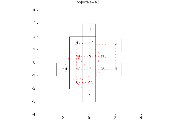
This example uses the convex-concave procedure to solve the problem of placing square circuit components on a chip to reduce the wirelength between them. Details can be found in section 5.3 of Variations and Extension of the Convex-Concave Procedure.

This example uses CVX, which is available here.

You can download the code circuit_placement_example.m, along with the two subroutines random_graph_generator.m and plot_circuits.m.

Contents

clear all
close all

Problem generation parameters

rand('state',0);
N = 15;% number of components
xbound = 4; % symmetric bounds on the bounding box in the x direction
ybound = 4; % symmetric bounds on the bounding box in the y direction
trials = 1; % number of initialization
rho = .4; % the chance any particular edge is in the graph
% a matrix with the height and width of each circuit component.
Circuits_size = ones(2,N);

Algorithm parameters

embedding_init = 0; % if 1, the first init. will be the Laplacian embedding
iterations = 150; % maximum number of iterations
Tau_init = 0.2;
Tau_inc = 1.1;
Tau_max = 1e4;

Laplacian embedding for an Erdos-Renyi random graph

L = random_graph_generator(N,rho);

% find the Laplacian embedding
if(embedding_init)
    [V D] = eig(L);
    i = 1;
    while(D(i,i) < 1e-8)
        i = i+1;
    end
    x = V(:,i);
    y = V(:,i+1);
    x = (x-((max(x)-min(x))/2+min(x)))/(max(x)-min(x));
    y = (y+((max(y)-min(y))/2+min(y)))/(max(x)-min(x));
    circuits = [2*xbound*x';2*ybound*y'];
end

Convex-concave procedure

figure
cvx_best = inf;
gradients = zeros(N*(N-1)/2,4);
constraint_val = zeros(N*(N-1)/2,1);

for Initialization = 1:trials
    %randomly initialize
    if(~embedding_init || Initialization~=1)
        circuits = [2*xbound 0; 0 2*ybound] *(rand(2,N)-.5);
    end
    %plot initial placement
    plot_circuits(circuits,Circuits_size,L,xbound,ybound,-1,-1,...
        Tau_init,Initialization)

    converge = 0; % flag to ensure two steps without change for convergence
    cvx_prev = inf;
    Tau = Tau_init;
    for k = 1:iterations
        circuits_c = circuits;
        % precalculate gradients
        for i = 1:N-1
            for j = i+1:N
                index = ((N-1)+(N-i+1))*(i-1)/2+j-i;
                % determine the vertical and horizontal margin on the
                % constraint.
                horiz = (Circuits_size(1,i)+Circuits_size(1,j))/2-...
                    abs(circuits_c(1,i)-circuits_c(1,j));
                vert =(Circuits_size(2,i)+Circuits_size(2,j))/2-...
                    abs(circuits_c(2,i)-circuits_c(2,j));
                %set which subgradient to use
                if(abs(horiz-vert) < 1e-5)
                    use = mod(k,2); % if the same alterante
                elseif(horiz < vert) % otherwise, go with the smaller
                    use = 0;
                else
                    use = 1;
                end
                if(use == 0)
                    s = sign(circuits_c(1,i)-circuits_c(1,j));
                    gradients(index,:) = [-s 0 s 0];
                else
                    s = sign(circuits_c(2,i)-circuits_c(2,j));
                    gradients(index,:) = [0 -s 0 s];
                end
                constraint_val(index) = min(horiz,vert);
            end
        end

        cvx_begin quiet
        variables circuits(2,N) slack(N*(N-1)/2)
        %the objective is the wire length between all connected
        %components.
        objective = 0;
        for i = 1:N-1
            for j = i+1:N
                if(L(i,j) < 0)
                    objective = objective + abs(circuits(1,i)-...
                        circuits(1,j)) + abs(circuits(2,i)-circuits(2,j));
                end
            end
        end
        minimize objective + Tau*(sum(slack))
        subject to
        %non overlapping constraint.
        for i = 1:N-1
            for j = i+1:N
                index = ((N-1)+(N-i+1))*(i-1)/2+j-i;
                constraint_val(index)+gradients(index,:)*...
                    ([circuits(1,i);
                    circuits(2,i);
                    circuits(1,j);
                    circuits(2,j)]-...
                    [circuits_c(1,i);
                    circuits_c(2,i);
                    circuits_c(1,j);
                    circuits_c(2,j)]) <= slack(index);
            end
        end
        slack >= 0;
        abs(circuits(1,:)) <= xbound-Circuits_size(1,:)./2;
        abs(circuits(2,:)) <= ybound-Circuits_size(2,:)./2;
        cvx_end

        %plot the resulting figure
        plot_circuits(circuits,Circuits_size,L,xbound,ybound,...
            objective,sum(slack),Tau,Initialization)

        if(norm(cvx_prev-cvx_optval) <= 1e-3 &&...
                (sum(slack) <= 1e-3 || Tau == Tau_max))
            if(converge == 1)
                break;
            else
                converge = 1;
            end
        else
            converge = 0;
        end

        Tau = min(Tau*Tau_inc,Tau_max);
        cvx_prev = objective + Tau*(sum(slack));

    end
    if(cvx_optval < cvx_best)
        cvx_best = cvx_optval;
        circuits_best = circuits;
    end
end


plot_circuits(circuits_best,Circuits_size,L,xbound,ybound,...
    cvx_best,-1,-1,-1,1)

Published with MATLAB® 7.10