fast_mpc: code for fast model predictive control
Version Alpha (Sep 2008)
Yang Wang and
Stephen Boyd
Purpose
fast_mpc contains two C functions, with MATLAB mex interface, that implement the fast model predictive control methods described in the paper Fast Model Predictive Control Using Online Optimization. See this paper for the precise problem formulation and meanings of the algorithm parameters.
Download and install
Get and unpack the package files from either of
This will create a directory that contains all source, as well as this documentation.
See the file INSTALL for installation instructions.
What fast_mpc does
We consider the control of a time-invariant linear dynamical system

where  ,
,  , and
, and  are the state, input, and disturbance
at time
are the state, input, and disturbance
at time  , and
, and  and
and  are the dynamics and input matrices.
In model predictive control (MPC), at each time we solve the QP
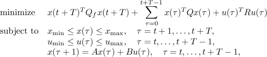
with variables

and data

The MPC input is  . We repeat this at the next time step.
fast_mpc is a software package for solving this optimization problem fast by exploiting its special structure, and by solving the problem approximately. The function fmpc_step solves the problem above, starting from a given initial state and input trajectory. The function fmpc_sim carries out a full MPC simulation of a dynamical system with MPC control.
Using fmpc_step
The function fmpc_step solves the above optimization problem and returns the
approximately optimal  and
and  trajectories. (In this case, you must
implement the MPC control loop yourself.) The calling procedure is as
follows.
trajectories. (In this case, you must
implement the MPC control loop yourself.) The calling procedure is as
follows.
[X,U,telapsed] = fmpc_step(sys,params,X0,U0,x0);
System description (sys structure):

    sys.A       :   dynamics matrix A
    sys.B       :   input matrix B
    sys.Q       :   state cost matrix Q
    sys.R       :   input cost matrix R
    sys.xmax    :   state upper limits x_{max}
    sys.xmin    :   state lower limits x_{min}
    sys.umax    :   input upper limits u_{max}
    sys.umin    :   input lower limits u_{min}
    sys.n       :   number of states
    sys.m       :   number of inputs

MPC parameters (params structure):

    params.T        :   MPC horizon T
    params.Qf       :   MPC final cost Q_f
    params.kappa    :   Barrier parameter
    params.niters   :   number of newton iterations
    params.quiet    :   no output to display if true

Other inputs
    X0   :   warm start X trajectory (n by T matrix)
    U0   :   warm start U trajectory (m by T matrix)
    x0   :   initial state

The inputs X0 and U0 need not satisfy the constraints; they are first
projected into the bounding box before the fast algorithm is applied.
X        :  optimal X trajectory (n by T matrix)
U        :  optimal U trajectory (m by T matrix)
telapsed :  time taken to solve the problem
Using fmpc_sim
The function fmpc_sim handles the entire MPC simulation.
For 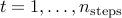 ,
fmpc_sim solves the above optimization problem, then applies the MPC input
and updates the state according to the dynamics equations.
The state and control trajectories are initialized with those from the
previous step, shifted in time, and
appending
,
fmpc_sim solves the above optimization problem, then applies the MPC input
and updates the state according to the dynamics equations.
The state and control trajectories are initialized with those from the
previous step, shifted in time, and
appending  and
and  , where

(As with fmpc_step, these trajectories are then projected into the
constraint box.)
Here  is the terminal control gain,

The calling procedure is
[Xhist,Uhist,telapsed] = fmpc_sim(sys,params,X0,U0,x0,w);
System description (sys structure):

    sys.A       :   dynamics matrix A
    sys.B       :   input matrix B
    sys.Q       :   state cost matrix Q
    sys.R       :   input cost matrix R
    sys.xmax    :   state upper limits x_{max}
    sys.xmin    :   state lower limits x_{min}
    sys.umax    :   input upper limits u_{max}
    sys.umin    :   input lower limits u_{min}
    sys.n       :   number of states
    sys.m       :   number of inputs

MPC parameters (params structure):

    params.T        :   MPC horizon T
    params.Qf       :   MPC final cost Q_f
    params.kappa    :   Barrier parameter
    params.niters   :   number of newton iterations
    params.quiet    :   no output to display if true
    params.nsteps   :   number of steps to run the MPC simulation

Other inputs
    X0   :   warm start X trajectory (n by T matrix)
    U0   :   warm start U trajectory (m by T matrix)
    x0   :   initial state
    w    :   disturbance trajectory (n by nsteps matrix)

The inputs X0 and U0 need not satisfy the constraints; they are first
projected into the bounding box before the fast algorithm is applied.
Xhist        :  state history (n by nsteps matrix)
Uhist        :  input history (m by nsteps matrix)
telapsed     :  time taken to solve the problem
Examples
We have provided two examples that illustrate usage:
masses_example.m uses fmpc_step to control a system of oscillating masses.
randsys_example.m uses fmpc_sim to simulate MPC on a randomly generated system.
Feedback
Please report any bugs to Yang Wang <yw224@stanford.edu>.
License
fast_mpc is under Apache license, version 2.0, January 2004.