Chapter 1
Introduction

1.1 WELCOME TO THE NEW PDP HANDBOOK

Several years ago, Dave Rumelhart and I first developed a handbook to introduce others to the parallel distributed processing (PDP) framework for modeling human cognition. When it was first introduced, this framwork represented a new way of thinking about perception, memory, learning, and thought, as well as a new way of characterizing the computational mechanisms for intelligent information processing in general. Since it was first introduced, the framework has continued to evolve, and it is still under active development and use in modeling many aspects of cognition and behavior.

Our own understanding of parallel distributed processing came about largely through hands-on experimentation with these models. And, in teaching PDP to others, we discovered that their understanding was enhanced through the same kind of hands-on simulation experience. The original edition of the handbook was intended to help a wider audience gain this kind of experience. It made many of the simulation models discussed in the two PDP volumes (Rumelhart et al., 1986; McClelland et al., 1986) available in a form that is intended to be easy to use. The handbook also provided what we hoped were accessible expositions of some of the main mathematical ideas that underlie the simulation models. And it provided a number of prepared exercises to help the reader begin exploring the simulation programs.

The current version of the handbook attempts to bring the older handbook up to date. Most of the original material has been kept, and a good deal of new material has been added. All of simulation programs have been implemented or re-implemented within the MATLAB programming environment. In keeping with other MATLAB projects, we call the suite of programs we have implemented the PDPTool software.

Although the handbook presents substantial background on the computational and mathematical ideas underlying the PDP framework, it should be used in conjunction with additional readings from the PDP books and other sources. In particular, those unfamiliar with the PDP framework should read Chapter 1 of the first PDP volume (Rumelhart et al., 1986) to understand the motivation and the nature of the approach.

This chapter provides some general information about the software and the handbook. The chapter also describes some general conventions and design decisions we have made to help the reader make the best possible use of the handbook and the software that comes with it. Information on how to set up the software (Appendix A), and a user’s guide (Appendix C), are provided in Appendices. At the end of the chapter we provide a brief tutorial on the MATLAB computing environment, within which the software is implemented.

1.2 MODELS, PROGRAMS, CHAPTERS AND EXCERCISES

The PDPTool software consists of a set of programs, all of which have a similar structure. Each program implements several variants of a single PDP model or network type. The programs all make use of the same interface and display routines, and most of the commands are the same from one program to the next.

Each program is introduced in a new chapter, which also contains relevant conceptual background for the type of PDP model that is encompassed by the program, and a series of excercises that allow the user to explore the properties of the models considered in the chapter.

In view of the similarity between the simulation programs, the information that is given when each new program is introduced is restricted primarily to what is new. Readers who wish to dive into the middle of the book, then, may find that they need to refer back to commands or features that were introduced earlier. The User’s Guide provides another means of learning about specific features of the programs.

1.2.1 Key Features of PDP Models

Here we briefly describe some of the key features most PDP models share. For a more detailed presentation, see Chapter 2 of the PDP book (Rumelhart et al., 1986).

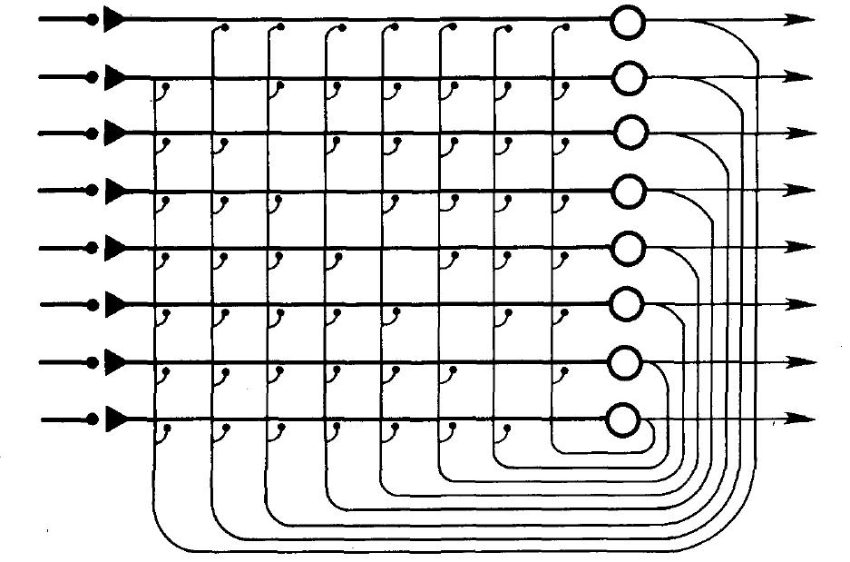
A PDP model is built around a simulated artificial neural network, which consists of units organized into pools, and connections among these units organized into projections. The minimal case (shown in Figure 2.1) would be a network with a single pool of units and a single projection from each unit in the network to every other unit. The basic idea is that units propagate excitatory and inhibitory signals to each other via the weighted connections. Adjustments may occur to the strengths of the connections as a result of processing. The units and connections constitute the architecture of the network, within which these processes occur. Units in a network may receive external inputs (usually from the network’s environment, described next), and outputs may be propagated out of the network.

A PDP model also generally includes an environment, which consists of patterns that are used to provide inputs and/or target values to the network. An input pattern specifies external input values for a pool of units. A target pattern specifies desired target activation values for units in a pool, for use in training the network. Patterns can be grouped in various ways to structure the input and target patterns presented to a network. Different groupings are used in different programs.

A PDP model also consists of a set of processes, including a test process and possibly a train process, as well as ancillary processes for loading, saving, displaying, and re-initializing. The test process presents input patterns (or sets of input patterns) to the network, and causes the network to process the patterns, possibly comparing the results to provided target patterns, and possibly computing other statistics and/or saving results for later inspection. Processing generally takes place in a single step or through a sequence of processing cycles. Processing consists of propagating activation signals from units to other units, multiplying each signal by the connection weight on the connection to the receiving unit from the sending unit. These weighted inputs are summed at the receiving unit, and the summed value is then used to adjust the activations of each recieving unit for the next processing step, according to a specified activation function. A train process presents a series of input patterns (or sets of input patterns), processes them using a process similar to the test process, then possibly compares the results generated to the values specified in target patterns (or sets of provided target patterns) and then carries out further processing steps that result in the adjustment of connections among the processing units.

The exact nature of the processes that take place in both training and testing are essential ingredients of specific PDP models and will be considered as we work through the set of models described in this book. The models described in Chapters 2 and 3 explore processing in networks with modeler-specified connection weights, while the models described in most of the later chapters involve learning as well as processing.

1.3 SOME GENERAL CONVENTIONS AND CONSIDERATIONS

1.3.1 Mathematical Notation

We have adopted a mathematical notation that is internally consistent within this handbook and that facilitates translation between the description of the models in the text and the conventions used to access variables in the programs. The notation is not always consistent with that introduced in the chapters of the PDP volumes or other papers. Here follows an enumeration of the key features of the notation system we have adopted. We begin with the conventions we have used in writing equations to describe models and in explicating their mathematical background.

Scalars.

Scalar (single-valued) variables are given in italic typeface. The names of parameters are chosen to be mnemonic words or abbreviations where possible. For example, the decay parameter is called decay.

Vectors.

Vector (multivalued) variables are given in boldface; for example, the external input pattern is called extinput. An element of such a vector is given in italic typeface with a subscript. Thus, the ith element of the external input is denoted extinput_i. Vectors are often members of larger sets of vectors; in this case, a whole vector may be given a subscript. For example, the jth input pattern in a set of patterns would be denoted ipattern_j.

Weight matrices.

Matrix variables are given in uppercase boldface; for example, a weight matrix might be denoted W. An element of a weight matrix is given in lowercase italic, subscripted first by the row index and then by the column index. The row index corresponds to the index of the receiving unit, and the column index corresponds to the index of the sending unit. Thus the weight to unit i from unit j would be found in the jth column of the ith row of the matrix, and is written w_ij.

Counting.

We follow the MATLAB language convention and count from 1. Thus if there are n elements in a vector, the indexes run from 1 to n. Time is a bit special in this regard. Time 0 (t₀) is the time before processing begins; the state of a network at t₀ can be called its “initial state.” Time counters are incremented as soon as processing begins within each time step.

1.3.2 Pseudo-MATLAB Code

In the chapters, we occasionally give pieces of computer code to illustrate the implementation of some of the key routines in our simulation programs. The examples are written in “pseudo-MATLAB”; details such as declarations are left out. Note that the pseudocode printed in the text for illustrating the implementation of the programs is generally not identical to the actual source code; the program examples are intended to make the basic characteristics of the implementation clear rather than to clutter the reader’s mind with the details and speed-up hacks that would be found in the actual programs.

Several features of MATLAB need to be understood to read the pseudo-MATLAB code and to work within the MATLAB environment. These are listed in the MATLAB mini-tutorial given at the end of this chapter. Readers unfamiliar with MATLAB will want to consult this tutorial in order to be able to work effectively with the PDPTool Software.

1.3.3 Program Design and User Interface

Our goals in writing the programs were to make them both as flexible as possible and as easy as possible to use, especially for running the core exercises discussed in each chapter of this handbook. We have achieved these somewhat contradictory goals as follows. Flexibility is achieved by allowing the user to specify the details of the network configuration and of the layout of the displays shown on the screen at run time, via files that are read and interpreted by the program. Ease of use is achieved by providing the user with the files to run the core exercises and by keeping the command interface and the names of variables consistent from program to program wherever possible. Full exploitation of the flexibility provided by the program requires the user to learn how to construct network configuration files and display configuration (or template) files, but this is only necessary when the user wishes to apply a program to some new problem of his or her own.

Another aspect of the flexibility of the programs is their permissiveness. In general, we have allowed the user to examine and set as many of the variables in each program as possible, including basic network configuration variables that should not be changed in the middle of a run. The worst that can happen is that the programs will crash under these circumstances; it is, therefore, wise not to experiment with changing them if losing the state of a program would be costly.

1.3.4 Exploiting the MATLAB Envioronment

It should be noted that the implementation of the software within the MATLAB environment provides two sources of further flexibility. First, users with a full MATLAB licence have access to the considerable tools of the MATLAB environment available for their use in perparing inputs and in analysing and visualizing outputs from simulations. We have provided some hooks into these visualization tools, but advanced users are likely to want to exploit some of the features of MATLAB for advanced analysis and visualization.

Second, because all of the source code is provided for all programs, it has proved fairly straightforward for users with some programming experience to delve into the code to modify it or add extensions. Users are encouraged to dive in and make changes. If you manage the changes you make carefully, you should be able to re-implement them as patches to future updates.

1.4 BEFORE YOU START

Before you dive into your first PDP model, we would like to offer both an exhortation and a disclaimer. The exhortation is to take what we offer here, not as a set of fixed tasks to be undertaken, but as raw material for your own explorations. We have presented the material following a structured plan, but this does not mean that you should follow it any more than you need to to meet your own goals. We have learned the most by experimenting with and adapting ideas that have come to us from other people rather than from sticking closely to what they have offered, and we hope that you will be able to do the same thing. The flexibility that has been built into these programs is intended to make exploration as easy as possible, and we provide source code so that users can change the programs and adapt them to their own needs and problems as they see fit.

The disclaimer is that we cannot be sure the programs are perfectly bug free. They have all been extensively tested and they work for the core exercises; but it is possible that some users will discover problems or bugs in undertaking some of the more open-ended extended exercises. If you have such a problem, we hope that you will be able to find ways of working around it as much as possible or that you will be able to fix it yourself. In any case, please let us how of the problems you encounter (Send bug reports, problems, and suggestions to Jay McClelland at mcclelland@stanford.edu). While we cannot offer to provide consultation or fixes for every reader who encounters a problem, we will use your input to improve the package for future users.

1.5 MATLAB MINI-TUTORIAL

Here we provide a brief introduction to some of the main features of the MATLAB computing environment. While this should allow readers to understand basic MATLAB operations, there are a many features of MATLAB that are not covered here. The built-in documentation in MATLAB is very thorough, and users are encouraged to explore the many features of the MATLAB environment after reading this basic tutorial. There are also many additional MATLAB tutorials and references available online; a simple Google search for ‘MATLAB tutorial’ should bring up the most popular ones.

1.5.1 Basic Operations

Comments. Comments in MATLAB begin with “%”. The MATLAB interpreter ignores anything to the right of the “%” character on a line. We use this convention to introduce comments into the pseudocode so that the code is easier for you to follow.

Variables. Addition (“+”), subtraction (“-”), multiplication (“*”), division (“/”), and exponentiation (“^”) on scalars all work as you would expect, following the order of operations. To assign a value to a variable, use “=”.

Note that MATLAB performs actual floating-point division, not integer division. Also note that MATLAB is case sensitive.

Displaying results of evaluating expressions. The MATLAB interpreter will evaluate any expression we enter, and display the result. However, putting a semicolon at the end of a line will suppress the output for that line. MATLAB also stores the result of the latest expression in a special variable called “ans”.

In general, MATLAB ignores whitespace; however, it is sensitive to line breaks. Putting “...” at the end of a line will allow an expression on that line to continue onto the next line.

1.5.2 Vector Operations

Building vectors Scalar values between “[” and “]” are concatenated into a vector. To create a row vector, put spaces or commas between each of the elements. To create a column vector, put a semicolon between each of the elements.

To transpose a vector (turning a row vector into a column vector, or vice versa), use “’”.

We can define a vector containing a range of values by using colon notation, specifying the first value, (optionally) an increment, and the last value.

We can get the length of a vector by using “length()”.

Accessing elements within a vector Once we have defined a vector and stored it in a variable, we can access individual elements within the vector by their indices. Indices in MATLAB start from 1. The special index ’end’ refers to the last element in a vector.

We can use colon notation in this context to select a range of values from the vector.

In fact, we can specify any arbitrary “index vector” to select arbitrary elements of the vector.

Furthermore, we can change a vector by replacing the selected elements with a vector of the same size. We can even delete elements from a vector by assigning the empty matrix “[]” to the selected elements.

Mathematical vector operations We can easily add (“+”), subtract (“-”), multiply (“*”), divide (“/”), or exponentiate (“.^”) each element in a vector by a scalar. The operation simply gets performed on each element of the vector, returning a vector of the same size.

Similarly, we can perform “element-wise” mathematical operations between two vectors of the same size. The operation is simply performed between elements in corresponding positions in the two vectors, again returning a vector of the same size. We use “+” for adding two vectors, and “-” to subtract two vectors. To avoid conflicts with different types of vector multiplication and division, we use “.*” and “./” for element-wise multiplication and division, respectively. We use “.^” for element-wise exponentiation.

Finally, we can perform a dot product (or inner product) between a row vector and a column vector of the same length by using (“*”). The dot product multiplies the elements in corresponding positions in the two vectors, and then takes the sum, returning a scalar value. To perform a dot product, the row vector must be listed before the column vector (otherwise MATLAB will perform an outer product, returning a matrix).

1.5.3 Logical operations

Relational operators We can compare two scalar values in MATLAB using relational operators: “==” (“equal to”), “~=” (“not equal to”), “<” (“less than”), “<=” (“less than or equal to”) “>” (“greater than”), and “>=” (“greater than or equal to”). The result is 1 if the comparison is true, and 0 if the comparison is false.

Note that floating-point comparisons work correctly in MATLAB.

The unary operator “~” (“not”) flips a binary value from 1 to 0 or 0 to 1.

Logical operations with vectors. As with mathematical operations, using a relational operator between a vector and a scalar will compare each each element of the vector with the scalar, in this case returning a binary vector of the same size. Each element of the binary vector is 1 if the comparison is true at that position, and 0 if the comparison is false at that position.

To test whether a binary vector contains any 1s, we use “any()”. To test whether a binary vector contains all 1s, we use “all()”.

We can use the binary vectors as a different kind of “index vector” to select elements from a vector; this is called “logical indexing”, and it returns all of the elements in the vector where the corresponding element in the binary vector is 1. This gives us a powerful way to select all elements from a vector that meet certain criteria.

1.5.4 Control Flow

Normally, the MATLAB interpreter moves through a script linearly, executing each statement in sequential order. However, we can use several structures to introduce branching and looping into the flow of our programs.

If statements. An if statement consists of: one if block, zero or more elseif blocks, and zero or one else block. It ends with the keyword end.

Any of the relational operators defined above can be used as a condition for an if statement. MATLAB executes the statements in an if block or a elseif block only if its associated condition is true. Otherwise, the MATLAB interpreter skips that block. If none of the conditions were true, MATLAB executes the statements in the else block (if there is one).

In fact, instead of using a relational operator as a condition, we can use any expression. If the expression evaluates to anything other than 0, the empty matrix [], or the boolean value false, then the expression is considered to be “true”.

While loops. A while loop works the same way as an if statement, except that, when the MATLAB interpreter reaches the end keyword, it returns to the beginning of the while block and tests the condition again. MATLAB executes the statements in the while block repeatedly, as long as the condition is true. A break statement within the while loop will cause MATLAB to skip the rest of the loop.

For loops. To execute a block of code a specific number of times, we can use a for loop. A for loop takes a counter variable and a vector. MATLAB executes the statements in the block once for each element in the vector, with the counter variable set to that element.

Although the “range” vector is most commonly a range of consecutive integers, it doesn’t have to be. Actually, the range vector doesn’t even need to be created with the colon operator. In fact, the range vector can be any vector whatsoever; it doesn’t even need to contain integers at all!

1.5.5 Vectorized Code

Vectorized code is code that describes (and, conceptually) executes mathematical operations on vectors an matrices “all at once”. Vectorised code is truer to the parallel “spirit” of the operations being performed in linear algebra, and also to the conceptual framework of PDP. Conceptually, the pseudocode descriptions of our algorithms (usually) should not involve the sequential repetition of a for loop. For example, when computing the input to a unit from other units, there is no reason for the multiplication of one activation times one connection weight to “wait” for the previous one to be completed. Instead, each multiplication should be though of as being performed independently and simultaneously. And in fact, vectorized code can execute much faster that code written explicitly as a for loop. This effect is especially pronounced when processing can be split across several processors.

Writing vectorised code. Let’s say we have two vectors, r and c.

We have seen two ways to perform a dot product between these two vectors. We can use a for loop:

However, the following “vectorized” code is more concise, and it takes advantage of MATLAB’s optimization for vector and matrix operations:

Similarly, we can use a for loop to multiply each element of a vector by a scalar, or to multiply each element of a vector by the corresponding element in another vector:

However, element-wise multiplication using .* is faster and more concise: