
In this chapter, we introduce a reinforcement learning method called Temporal-Difference (TD) learning. Many of the preceding chapters concerning learning techniques have focused on supervised learning in which the target output of the network is explicitly specified by the modeler (with the exception of Chapter 6 Competitive Learning). TD learning is an unsupervised technique in which the learning agent learns to predict the expected value of a variable occurring at the end of a sequence of states. Reinforcement learning (RL) extends this technique by allowing the learned state-values to guide actions which subsequently change the environment state. Thus, RL is concerned with the more holistic problem of an agent learning effective interaction with its environment. We will first describe the TD method for prediction, and then extend this to a full conceptual picture of RL. We then explain our implementation of the algorithm to facilitate exploration and solidify an understanding of how the details of the implementation relate to the conceptual level formulation of RL. The chapter concludes with an excercise to help fortify understanding.
To borrow an apt example from Sutton (1988), imagine trying to predict Saturday’s weather at the beginning of the week. One way to go about this is to observe the conditions on Monday (say) and pair this observation with the actual meteorological conditions on Saturday. One can do this for each day of the week leading up to Saturday, and in doing so, form a training set consisting of the weather conditions on each of the weekdays and the actual weather that obtains on Saturday. Recalling Chapter 5, this would be an adequate training set to train a network to predict the weather on Saturday. This general approach is called supervised learning because, for each input to the network, we have explicily (i.e. in a supervisory manner) specified a target value for the network. Note, however, that one must know the actual outcome value in order to train this network to predict it. That is, one must have observed the actual weather on Saturday before any learning can occur. This proves to be somewhat limiting in a variety of real-world scenarios, but most importantly, it seems a rather inefficient use of the information we have leading up to Saturday. Suppose, for instance, that it has rained persistently throughout Thursday and Friday, with little sign that the storm will let up soon. One would naturally expect there to be a higher chance of it raining on Saturday as well. The reason for this expectation is simply that the weather on Thursday and Friday are relevant to predicting the weather on Saturday, even without actually knowing the outcome of Saturday’s weather. In other words, partial information relevant to our prediction for Saturday becomes available on each day leading up to it. In supervised learning as it was previously described, this information is effectively not employed in learning because Saturday’s weather is our sole target for training.
Unsupervised learning, in contrast, operates instead by attempting to use intermediate information, in addition to the actual outcome on Saturday, to learn to predict Saturday’s weather. While learning on observation-outcome pairs is effective for predictions problems with only a single step, pairwise learning, for the reason motivated above, is not well suited to prediction problems with multiple steps. The basic assumption that underlies this unsupervised approach is that predictions about some future value are ”not confirmed or disconfirmed all at once, but rather bit by bit” as new observations are made over many steps leading up to observation of the predicted value (Sutton, 1988). (Note that, to the extent that the outcome values are set by the modeler, TD learning is not unsupervised. We use the terms ’supervised’ and ’unsupervised’ here for convenience to distinguished the pairwise method from the TD method, as does Sutton. The reader should be aware that the classification of TD and RL learning as unsupervised is contested.)
While there are a variety of techniques for unsupervised learning in prediction problems, we will focus specifically on the method of Temporal-Difference (TD) learning (Sutton, 1988). In supervised learning generally, learning occurs by minimizing an error measure with respect to some set of values that parameterize the function making the prediction. In the connectionist applications that we are interested in here, the predicting function is realized in a neural network, the error measure is most often the difference between the output of the predicting function and some prespecificed target value, and the values that parameterize the function are connection weights between units in the network. For now, however, we will dissociate our discussion of the prediction function from the details of its connectionist implementation for the sake of simplicity and because the principles which we will explore can be implemented by methods other than neural networks. In the next section, we will turn our attention to understanding how neural networks can implement these prediction techniques and how the marriage of the two techniques (TD and connectionism) can provide added power.
The general supervised learning paradigm can be summarized in a familiar formula
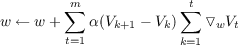
where wt is a vector of the parameters of our prediction function at time step t, α is a learning rate constant, z is our target value, V (st) is our prediction for input state st, and ▿wV (st) is the vector of partial derivatives of the prediction with respect to the parameters w. We call the function, V (⋅), which we are trying to learn, the value function. This is the same computation that underlies back propagation, with the amendment that wt are weights in the network and the back propagation procedure is used to calculate the gradient ▿wV (st). As we noted earlier, this update rule cannot be computed incrementally with each step in a multi-step prediction problem because the value of z is unknown until the end of the sequence. Thus, we are required to observe a whole sequence before updating the weights, so the weight update for an entire sequence is just the sum of the weight changes for each time step,
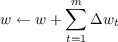
where m is the number of steps in the sequence.
The insight of TD learning is that the error, z - V t, at any time can be represented as the sum of changes in predictions on adjacent time steps, namely
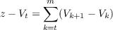
where V t is shorthand for V (st), V m+1 is defined as z, and sm+1 is the terminal state in the sequence. The validity of this formula can be verified by merely expanding the sum and observing that all terms cancel, leaving only z - V t.
Thus, substituting for Δwt in the sequence update formula we have
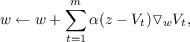
and substituting the sum of differences for the error, (z - V t), we have,
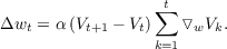
After some algebra, we obtain
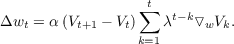
from which we can extract the weight update rule for a single time step by noting that the term inside the first sum is equivalent to Δwt by comparison to the sequence update equation,
It is worth pausing to reflect on how this update rule works mechanistically. We need two successive predictions to form the error term, so we must already be in state st+1 to obtain our prediction V t+1, but learning is occurring for prediction V t (i.e. wt is being updated). Learning is occuring retroactively for already visited states. This is accomplished by maintaining the gradient ▿wV k as a running sum. When the error appears at time t + 1, we obtain the appropriate weight changes for updating all of our predictions for previous input states by multiplying this error by the summed gradient. The update rule is, in effect, updating all preceding predictions to make each closer to prediction V t+1 for the current state by using the difference in the successive prediction values, hence the name Temporal-Difference learning.
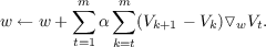
This update rule will produce the same weight changes over the sequence as the supervised version will (recall that we started with the supervised update equation for a sequence in the derivation), but this rule allows weight updates to occur incrementally - all that is necessary is a pair of successive predictions and the running sum of past output gradients. Sutton (1988) calls this the TD(1) procedure and introduces a generalization, called TD(λ), which produces weight changes that supervised methods cannot produce. The generalized formula for TD(λ) is
We have added a constant, λ, which exponentially discounts past gradients. That is, the gradient of a prediction occurring n steps in the past is weighted by λn. Naturally, λ lies in the interval [0,1]. We have seen that λ = 1 produces the same weight changes as a supervised method that uses observation-outcome pairs as its training set. Setting λ = 0 results in the formula

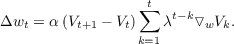
This equation is equivalent to the the supervised learning rule with V t+1 substituted for z. Thus, TD(0) produces the same weight changes as would a supervised method whose training pairs are simply states and the predictions made on the immediately follow state, i.e. training pairs consist of st as input and V t+1 as target. Conceptually, intermediate values of λ result in an update rule that falls somewhere between these two extremes. Specifically, λ determines the extent to which the prediction values for previous observations are updated by errors occuring on the current step. In other words, it tracks to what extent previous predictions are eligible for updating based on current errors. Therefore, we call the sum,
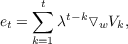
the eligibility trace at time t. Eligibility traces are the primary mechanisms of temporal credit assignment in TD learning. That is, credit (or “blame”) for the TD error occurring on a given step is assigned to the previous steps as determined by the eligibility trace. For high values of λ, predictions occurring earlier in a sequence are updated to a greater extent than with lower values of λ for a given error signal on the current step.
To consider an example, suppose we are trying to learn state values for the states in some sequence. Let us refer to states in the sequence by letters of the alphabet. Our goal is to learn a function V (⋅) from states to state-values. State-values approximate the expected value of the variable occuring at the end of the sequence. Suppose we initialize our value function to zero, as is commonly done (it is also common to initialize them randomly, which is natural in the case of neural networks). We encounter a series of states such as a, b, c, d. Since predictions for these values is zero at the outset, no useful learning will occur until we encounter the outcome value at the end of the sequence. Nonetheless, we find the output gradient for each input state and maintain the eligibility trace as a discounted sum of these gradients. Suppose that this particular sequence ends with z = 1 at the terminal state. Upon encountering this, we have a useful error as our training signal, z - V (d). After obtaining this error, we multiply it by our eligibility trace to obtain the weight changes. In applying these weight changes, we correct the predictions of all past states to be closer to the value at the end of the sequence, since the eligibility trace includes the gradient for past states. This is desirable since all of the past states in the sequence led to an outcome of 1. After a few such sequences, our prediction values will no longer be random. At this point, valuable learning can occur even before a sequence ends. Suppose that we encounter states c and then b. If b already has a high (or low) value, then the TD error, V (b) - V (c) will produce an appropriate adjustment in V (c) toward V (b). In this way, TD learning is said to bootstrap in that it employs its own value predictions to correct other value predictions. One can think of this learning process as the propagation of the outcome value back through the steps of the sequence in the form of value predictions. Note that this propagation occurs even when λ = 0, although higher values of λ will speed the process. As with supervised learning, the success of TD learning depends on passes through many sequences, although learning will be more efficient in general.
Now we are in a state to consider how it is exactly that TD errors can drive more efficient learning in prediction problems than its supervised counterpart. After all, with supervised learning, each input state is paired with the actual value that it is trying to predict - how can one hope to do better than training on veridical outcome information? Figure 9.1 illustrates a scenario in which we can do better. Suppose that we are trying to learn the value function for a game. We have learned thus far that the state labeled BAD leads to a loss 90% of the time and a win 10% of the time, and so we appropriately assign it a low value. We now encounter a NOVEL state which leads to BAD but then results in a win. In supervised learning, we would construct a NOVEL-win training pair and the NOVEL state would be initially assigned a high value. In TD learning, the NOVEL state is paired with the subsequent BAD state, and thus TD assigns the NOVEL state a low value. This is, in general, the correct conclusion about the NOVEL state. Supervised methods neglect to account for the fact that the NOVEL state ended in a win only by transitioning through a state that we already know to be bad. With enough training examples, supervised learning methods can acheive equivalent performance, but TD methods make more efficient use of training data in multi-step prediction problems by bootstrapping in this way and so can learn more efficiently with limited experience.
So far we have seen how TD learning can learn to predict the value of some variable over multiple time steps - this is the prediction problem. Now we will address the control problem, i.e. the problem of getting an RL agent to learn how to control its environment. The control problem is often considered to be the complete reinforcement learning problem in that the agent must learn to both predict the values of environment states that it encounters and also use those predicted values to change the environment in order to maximize reward. In this section, we introduce the framework for understanding the full RL problem. Later, we present a case study of combining TD learning with connectionist networks.
We now introduce a slight change in terminology with an accompanying addition to the concept of predicting outcomes that we explored in the previous section. We will hereafter refer to the outcome value of a sequence as the reward. Since we will consider cases in which the learning agent is trying to maximize the value of the outcome, this shift in terminology is natural. Rewards can be negative as well as positive - when they are negative they can be thought of as punishment. We can easily generalize the TD method to cases where there are intermediate reward signals, i.e. reward signals occuring at some state in the sequence other than the terminal state. We consider each state in a sequence to have an associated reward value, although many states will likely have a reward of 0. This transforms the prediction problem from one of estimating the expected value of a reward occurring at the end of a sequence to one of estimating the expected value of the sum of rewards encountered in a sequence. We call this sum of rewards the return. Using the sum of rewards as the return is fine for tasks which can be decomposed into distinct episodes. However, to generalize to tasks which are ongoing and do not decompose into episodes, we need a means by which to keep the return value bounded. Here we introduce the discounting parameter, gamma, denoted γ. Our total discounted return is given by
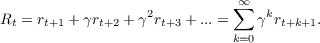
Discounting simply means that rewards arriving futher in the future are worth less. Thus, for lower values of γ, distal rewards are valued less in the value prediction for the current time. The addition of the γ parameter not only generalizes TD to non-episodic tasks, but also provides a means by which to control how far the agent should look ahead in making predictions at the current time step.
We would like our prediction V t to approximate Rt, the expected return at time t. Let us refer to the correct prediction for time t as V t*; so V t* = Rt. We can then derive the generalized TD error equation from the right portion of the return equation.
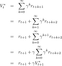
We note that the TD error at time t will be Et = V t*-V t and we use V t+1 as an imperfect proxy for the true value V t+1* (bootstrapping). We substitute to obtain the generalized error equation:

This error will be multiplied by a learning rate α and then used to update our weights. The general update rule is
![Vt ← Vt + α[rt+1 + γVt+1 - Vt]](handbook122x.png)
Recall, however, that when using the TD method with a function approximator like a neural network, we update V t by finding the output gradient with respect to the weights. This step is not captured in the previous equation. We will discuss these implementation specific details later.
It is worthwhile to note that the return value provides a replacement for planning. In attaining some distal goal, we often thing that an agent must plan many steps into the future to perform the correct sequence of actions. In TD learning, however, the value function V t is adjusted to reflect the total expected return after time t. Thus, in considering how to maximize total returns in making a choice between two or more actons, a TD agent need only choose the action with the highest state value. The state values themselves serve as proxies for the reward value occurring in the future. Thus, the problem of planning a sequence of steps is reduced to the problem of choosing a next state with a high state value. Next we explore the formal characterization of the full RL problem.
In specifying the control problem, we divide the agent-environment interaction into conceptually distinct modules. These modules serve to ground a formal characterization of the control problem independent of the details of a particular environment, agent, or task. Figure 9.2 is a schematic of these modules as they relate to one another. The environment provides two signals to the agent: the current environment state, st, which can be thought of as a vector specifying all the information about the environment which is available to the agent; and the reward signal, rt, which is simply the reward associated with the co-occurring state. The reward signal is the only training signal from the environment. Another training signal is generated internally to the agent: the value of the successor state needed in forming the TD error. The diagram also illustrates the ability of the agent to take an action on the environment to change its state.

Note that the architecture of a RL agent is abstract: it need not align with actual physical boundaries. When thinking conceptually about an RL agent, it is important to keep in mind that the agent and environment are demarcated by the limits of the agent’s control (Sutton and Barto, 1998). That is, anything that cannot be arbitrarily changed by the agent is considered part of the agent’s environment. For instance, although in many biological contexts the reward signal is computed inside the physical bounds of the agent, we still consider them as part of the environment because they cannot be trivially modified by the agent. Likewise, if a robot is learning how to control its hand, we should consider the hand as part of the environment, although it is physically continuous with the robot.
We have not yet specified how action choice occurs. In the simplest case, the agent evaluates possible next states, computes a state value estimate for each one, and chooses the next state based on those estimates. Take, for instance, an agent learning to play the game Tic-Tac-Toe. There might be a vector of length nine to represent the board state. When it is time for the RL agent to choose an action, it must evaluate each possible next state and obtain a state value for each. In this case, the possible next states will be determined by the open spaces where an agent can place its mark. Once a choice is made, the environment is updated to reflect the new state.
Another way in which the agent can modify its environment is to learn state-action values instead of just state values. We define a function Q(⋅) from state-action pairs to values such that the value of Q(st,at) is the expected return for taking action at while in state st. In neural networks, the Q function is realized by having a subset of the input units represent the current state and another subset represent the possible actions. For the sake of illustration, suppose our learning agent is a robot that is moving around a grid world to find pieces of garbage. We may have a portion of the input vector to represent sensory information that is available to the robot at its current location in the grid - this portion corresponds to the state in the Q function. Another portion would be a vector for each possible action that the robot can take. Suppose that our robot can go forward, back, left, right, and pickup a piece of trash directly in front of it. Therefore, we would have a five place action vector, one place corresponding to each of the possible actions. When we must choose an action, we simply fix the current state on the input vector and turn on each of the five action units in turn, computing the value for each. The next action is chosen from these state-action values and the environment state is modified accordingly.
The update equation for learning state-action values is the same in form as that of learning state values which we have already seen:
![Q(s ,a) ← Q(s ,a)+ α [r + γQ(s ,a )- Q (s ,a )].
t t t t t+1 t+1 t+1 t t](handbook123x.png)
This update rule is called SARSA for State Action Reward State Action because it uses the state and action of time t along with the reward, state, and action of time t + 1 to form the TD error. This update rule is called associative because the values that it learns are associated with particular states in the environment. We can write the same update rule without any s terms. This update rule would learn the value of actions, but these values would not be associated with any environment state, thus it is nonassociative. For instance, if a learning agent were playing a slot machine with two handles, it would be learning only action values, i.e. the value of pulling lever one versus pulling lever two. The associative case of learning state-action values is commonly thought of as the full reinforcement learning problem, although the related state value and action value cases can be learned by the same TD method.
Action choice is specified by a policy. A policy is considered internal to the agent and consists of a rule for choosing the next state based on the value predictions for possible next states. More specifically, a policy maps state values to actions. Policy choice is very important due to the need to balance exploration and exploitation. The RL agent is trying to accomplish two related goals at the same time: it is trying to learn the values of states or actions and it is trying to control the environment. Thus, initially the agent must explore the state space to learn approximate value predictions. This often means taking suboptimal actions in order to learn more about the value of an action or state. Consider an agent who takes the highest-valued action at every step. This policy is called a greedy policy because the agent is only exploiting its current knowledge of state or action values to maximize reward and is not exploring to improve its estimates of other states. A greedy policy is likely undesirable for learning because there may be a state which is actually good but whose value cannot be discovered because the agent currently has a low value estimate for it, precluding its selection by a greedy policy. Furthermore, constant exploratory action is necessary in nonstationary tasks in which the reward values actually change over time.
A common way of balancing the need to explore states with the need to exploit current knowledge in maximizing rewards is to follow an ε-greedy policy which simply follows a greedy policy with probabiliy 1 - ε and takes a random action with probability ε. This method is quite effective for a large variety of tasks. Another common policy is softmax. You may recognize softmax as the stochastic activation function for Boltzmann machines introduced in Chapter 3 on Constraint Satisfaction - it is often called the Gibbs or Boltzmann distribution. With softmax, the probability of choosing action a at time t is
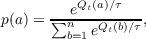
where the denominator sums over all the exponentials of all possible action values and τ is the temperature coefficient. A high temperature causes all actions to be equiprobable, while a low temperature skews the probability toward a greedy policy. The temperature coefficient can also be annealed over the course of training, resulting in greater exploration at the start of training and greater exploitation near the end of training. All of these common policies are implemented in the pdptool software, along with a few others which are documented in Section 9.5.
As mentioned previously, TD methods have no inherent connection to neural network architectures. TD learning solves the problem of temporal credit assignment, i.e. the problem of assigning blame for error over the sequence of predictions made by the learning agent. The simplest implementation of TD learning employs a lookup table where the value of each state or state-action pair is simply stored in a table, and those values are adjusted with training. This method is effective for tasks which have an enumerable state space. However, in many tasks, and certainly in tasks with a continuous state space, we cannot hope to enumerate all possible states, or if we can, there are too many for a practical implementation. Back propagation, as we already know, solves the problem of structural credit assignment, i.e. the problem of how to adjust the weights in the network to minimize the error. One of the largest benefits of neural networks is, of course, their ability to generalize learning across similar states. Thus, combining both TD and back propagation results in an agent that can flexibly learn to maximize reward over mulitple time steps and also learn structural similarities in input patterns that allow it to generalize its predictions over novel states. This is a powerful coupling. In this section we sketch the mathematical machinery involved in coupling TD with back propagation. Then we explore a notable application of the combined TDBP algorithm to the playing of backgammon as a case study.
As we saw in the beginning of this chapter, the gradient descent version of TD learning can be described by the general equation reproduced below:
The key difference between regular back propagation and TD back propagation is
that we must adjust the weights for the input at time t at time t + 1. This requires
that we compute the output gradient with respect to weights for input at time t and
save this gradient until we have the TD error at time t + 1. Just as in regular back
propagation, we use the logistic activation function, f(neti) =  , where
neti is the net input coming into output unit i from a unit j that projects to it.
Recall that the derivative of the activation function with respect to net input is
simply
, where
neti is the net input coming into output unit i from a unit j that projects to it.
Recall that the derivative of the activation function with respect to net input is
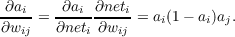
simply  = f′(neti) = ai(1 -ai), where ai is the activation at output unit i, and
the derivative of the net input neti with respect to the weights is
= f′(neti) = ai(1 -ai), where ai is the activation at output unit i, and
the derivative of the net input neti with respect to the weights is  = aj. Thus,
the output gradient with respect to weights for the last layer of weights
is
= aj. Thus,
the output gradient with respect to weights for the last layer of weights
is
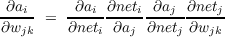
Similarly, the output gradient for a weight from unit k to unit j is
We have seen all of this before in Chapter 5. But now, we use δik to
denote  , where k is a hidden layer unit and i is an output unit. By using
the chain rule, we can calculate a δ term for each hidden layer. δii for the
output layer is simply ai(1 - ai). The δ term for any hidden unit k is given
by
, where k is a hidden layer unit and i is an output unit. By using
the chain rule, we can calculate a δ term for each hidden layer. δii for the
output layer is simply ai(1 - ai). The δ term for any hidden unit k is given
by
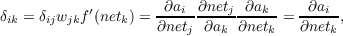
where j is a unit in the next layer forward and δij has already been computed for that layer. This defines the back propagation process that we must use. Note the difference between this calculation and the similar calculation of δ terms introduced in Chapter 5: in regular back propagation, the δi at the output is (ti - ai)f′(neti). Thus, in regular back propagation, the error term is already multiplied into the δ term for each layer. This is not the case in TDBP because we do not yet have the error. This means that, in general, the δ term for any hidden layer will be a two dimensional matrix of size i by k where i is the number of output units and k is the number of units at the hidden layer. In the case of the output layer, the δ term is just a vector of length i.
We use the δ terms at each layer to calculate the output gradient with respect to the weights by simply multiplying it by the activation of the projecting layer:
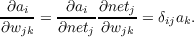
In general, this will give us a three dimensional matrix for each weight projection wjk of size i by j by k where element (i,j,k) is the derivative of output unit i with respect to the weight from unit k to unit j. This gradient term is scaled by λ and added to the accumulating eligibility trace for that projection. Thus, eligibility traces are three dimensional matrices denoted by eijk. Upon observing the TD error at the next time step, we compute the appropriate weight changes by
where Ei is the TD error at output unit i.
In regular back propagation, for cases where a hidden layer projects to more than one layer, we can calculate δ terms back from each output layer and simply sum them to obtain the correct δ for the hidden layer. This is because the error is already multiplied into the δ terms, and they will simply be vectors of the same size as the number of units in the hidden layer. In our implementation of TDBP, however, the δ term at a hidden layer that projects to more than one layer is the concatenation of the two δ matrices along the i dimension (naturally, this is true of the eligibility trace at that layer as well). The TD error for that layer is similarly a vector of error terms for all output units that the layer projects to. Thus, we obtain the correct weight changes for networks with multiple paths to the output units.

Backgammon, briefly, is a board game which consists of two players alternately rolling a pair of dice and moving their checkers opposite directions around the playing board. Each player has fifteen checkers distributed on the board in a standard starting position illustrated in Figure 9.3. On each turn, a player rolls and moves one checker the number shown on one die and then moves a second checker (which can be the same as the first) the number shown on the other die. More than one of a player’s checkers can occupy the same place on the board, called a “point.” If this is the case, the other player cannot land on the point. However, if there is only one checker on a point, the other player can land on the point and take the occupying checker off the board. The taken pieces are placed on the “bar”, where they must be reentered into the game. The purpose of the game is to move each of one’s checkers all the way around and off the board. The first player to do this wins. If a player manages to remove all her pieces from the board before the other player has removed any of his pieces, she is said to have won a “gammon,” which is worth twice a normal win. If a player manages to remove all her checkers and the other player has removed none of his and has checkers on the bar, then she is said to have won a “backgammon,” which is worth three times a normal win. The game is often played in matches and can be accompanied by gambling.
The game, like chess, has been studied intently by computer scientists. It has a very large branching rate: the number of moves available on the next turn is very high due to the high number of possible dice rolls and the many options for disposing of each roll. This limits tree search methods from being very effective in programming a computer to play backgammon. The large number of possible board positions also precludes effective use of lookup tables. Gerald Tesauro at IBM in the late 80’s was the first to successfully apply TD learning with back propagation to learning state values for backgammon (Tesauro, 1992).
Tesauro’s TD-Gammon network had an input layer with the board representation and a single hidden layer. The output layer of the network consisted of four logistic units which estimate the probability of white or black both achieving a regular win or a gammon. Thus, the network was actually estimating four outcome values at the same time. The input representation in the first version of TD-Gammon was 198 units. The number of checkers on each of the 24 points on the board were represented by 8 units. Four of the units were devoted to white and black respectively. If one white checker was on a given point, then the first unit of the four was on. If two white checkers were on a given point, then both the first and second unit of the group of four were on. The same is true for three checkers. The fourth unit took on a graded value to represent the number of checkers above three: (n∕2), where n is the number of checkers above three. In addition to these units representing the points on the board, an additional two units encoded how many black and white checkers were on the bar (off the board), each taking on a value (n∕2), where n is the number of black/white checkers on the bar. Two more units encoded how many of each player’s checkers had already been removed from the board, taking on values of (n∕15), where n is the number of checkers already removed. The final two units encoded whether it was black or white’s turn to play. This input projected to a hidden layer of 40 units.
Tesauro’s previous backgammon network, Neurogammon, was trained in a supervised manner on a corpus of expert level games. TD-Gammon, however, trained by completely by self-play. Moves were generated by the network itself in the following fashion: the computer simulated a dice roll and generated all board positions that were possible from the current position and the number of the die. The network was fed each of these board positions and the one that the network ranked highest was chosen as the next state. The network then did the same for the next player and so on. Initially, the network chose moves randomly because its weights were initialized randomly. After a sufficient number of games, the network played with more direction, allowing it to explore good strategies in greater depth. The stochastic nature of backgammon allowed the network to thoroughly explore the state space. This self-play learning regime proved effective against Neurogammon’s supervised technique.
The next generation of TD-Gammon employed a different input representation that included a set of conceptual features that are relevent to experts. For instance, units were added to encode the probability of a checker being hit and the relative strength of blockades (Tesauro, 2002). With this augmentation of the raw board position, TD-Gammon acheived expert-level play and is still widely regarded as the best computerized player. It is commonly used to analyze games and evaluate the quality of decisions by expert players. Thus, the input representation to TDBP networks is an important consideration when building a network.
There are other factors contributing to the success that Tesauro achieved with TD-Gammon (Tesauro, 1992). Notably, backgammon is a non-deterministic game. Therefore, it has a relatively smooth and continuous state space. This means simply that similar board positions have similar values. In deterministic games, such as chess, a small difference in board position can have large consequences for the state value. Thus, the sort of state value generalization in TD-Gammon would not be as effective and the discontinuities in the chess state space would be harder to learn. Similarly, a danger with learning by self-play is that the network will learn a self-consistent strategy in which it performs well in self-play, but performs poorly against other opponents. This was remedied largely by the stochastic nature of backgammon which allowed good coverage of the state space. Parameter tuning was largely done heuristically with λ = 0.7 and α = 0.1 for much of the training. Decreases in λ can help focus learning after the network has become fairly proficient at the task, but these parameter settings are largely the decision of the modeler and should be based on specific considerations for the task at hand.
The tdbp program implements the TD back propagation algorithm. The structure of the program is very similar to that of the bp program. Just as in the bp program, pool(1) contains the single bias unit, which is always on. Subsequent pools must be declared in the order of the feedforward structure of the network. Each pool has a specified type: input, hidden, output, and context. There can be one or more input pools and all input pools must be specified before any other pools. There can be zero or more hidden pools and all hidden pools must be specified before output pools but after input pools. There can be one or more output pools, and they are specified last. There are two options for output activation function: logistic and linear. The logistic activation function, as we have seen in earlier chapters, ranges between 0 and 1 and has a natural interpretation as a probability for binary outcome tasks. The linear activation function is equivalent to the net input to the output units. The option of a linear activation function provides a means to learn to predict rewards that do not fall in the range of 0 to 1. This does not exclude the possibility of using rewards outside that range with the logisitic activation function - the TD error will still be generated correctly, although the output activation can never take on values outside of [0, 1]. Lastly, context pools are a special type of hidden pool that operate in the same way as in the srn program.
The gamma parameter can be set individually for each output pool, and if this value it unspecified, the network-wide gamma value is used. Output units also have an actfunction parameter which takes values of either ’logistic’ or ’linear’. Each pool also has a delta variable and an error variable. As mentioned previously, the delta value will, in general, be a two dimensional matrix. The error variable simply holds the error terms for each output unit that lies forward from the pool in the network. Thus, it will not necessarily be of the same size as the number of units in the pool, but it will be the same size as the first dimension of the delta matrix. Neither the error nor the delta parameter is available for display in the network window although both can be printed to the console since they are fields of the pool data structure.
Projections can be between any pool and a higher numbered pool. The bias pool can project to any pool, although projections to input pools will have no effect because the units of input pools are clamped to the input pattern. Context pools can receive a special type of copyback projection from another hidden pool, just as in the srn program. Projections from a layer to itself are not allowed. Every projection has an associated eligibility trace, which is not available for display in the network display since, in general, it is a three dimensional matrix. It can, however, be printed to the console and is a field of the projection data structures in the net global variable called eligtrace. Additionally, each projection has a lambda and lrate parameter which specify those values for that projection. If either of these parameters is unspecified, the network-wide lambda and lrate values are used.
There are two modes of network operation - “beforestate” or “afterstate” - which are specified in the .net file of the network when the network is created. In “beforestate” mode, the tdbp program (1) presents the current environment state as the network input, (2) performs weight changes, (3) obtains and evaluates possible next states, and (4) sets the the next state. In contrast, the “afterstate” mode instructs the tdbp program to (1) obtain and evaluate possible next states, (2) set the selected state as input to the network, (3) perform weight changes, and (4) set the next state. In both cases, learning only occurs after the second state (since we need two states to compute the error). For simple prediction problems, in which the network does not change the state of the environment, the “beforestate” mode is usually used. For any task in which the network modifies the environment, “afterstate” is likely the desired mode. Any SARSA learning should use the “afterstate” mode. Consider briefly why this should be the case. If the agent is learning to make actions, then in “afterstate” mode it will first choose which action to take in the current state. Its choice will then be incorporated into the eligibility trace for that time step. Then the environment will be changed according to the network choice. This new state will have an associated reward which will drive learning on the next time step. Thus, this new reward will be the result of taking the selected action in the associated state, and learning will correctly adjust the value of the initial state-action pair by this new reward. In other words, the reward signal should follow the selection of an action for learning state-action pairs. If you are learning to passively predict, or learning a task in which states are selected directly, then the pre-selection of the next state is unnecessary.
The largest difference between the tdbp program and the bp program is that a Matlab class file takes the place of pattern files. As an introductory note, a class is a concept in object-oriented programming. It specifies a set of properties and methods that a virtual object can have. Properties are simply variables belonging to the object and methods are functions which the object can perform. To provide a simple example, we might wish to define a class called ’dog.’ The dog class might have a property specifying, e.g., the frequency of tail wags and a method called ’fetch.’ This class is said to be instantiated when a dog object is created from it. An instantiated class is called an ’object’ or ’instance’ and it differs from a class in that it owns its own properties and methods. So we might instantiate many dog objects, each with different frequency of tail wagging. Thus, a class specifies a data structure and an object is a discrete instance of that data structure. For more information about object-orient programming in Matlab, please consult the Matlab Object-Oriented User Guide (http://www.mathworks.com/help/techdoc/matlab_oop/ug_intropage.html).
Matlab class files are Matlab .m files that specify a Matlab object which has both data fields, like a data structure, and methods, which provide functionality. We call this class file an “environment class.” The environment class is specified by the modeler to behave in a functionally equivalent way to the task environment that the modeler wishes to model. The environment class provides all input patterns to the network, all reward signals, and all possible next states for the network to evaluate. As such, environment classes must adhere to a standard interface of methods and properties so that it can interact with the tdbp program. The envir_template.m file is a skeletal specification of this standard interface. The environment class file is specified to pdptool just as .pat files are in the bp program. You can select an environment file (with .m extension) in the pattern selection dialogue box by clicking the Load Pattern button in the main pdp window and changing the file type to .m. The tdbp program instantiates the class as an object named “envir,” which is a global variable in the workspace, just like the “net” variable. We will briefly review the functionality of the environment class, but please refer to the envir_template.m file for a full explanation of the requisite functionality. It is recommended that a modeler wishing to create his own environment class use the template file as a start.
The interface for the environment class specifies one property and ten methods, two of which are optional. The required property is a learning flag, lflag. Note that the tdbp program has its own lflag which can be set in the training options dialogue. If either of these variables is equal to 0, the network will skip training (and computing eligibilities) for the current time step. This allows you to control which steps the network takes as training data from within your environment class, which is particularly useful for game playing scenarios in which the network makes a move and then the game state is inverted so that the network can play for the other side. We only want to train the network on a sequence of states which only one of the players would have to play. Otherwise, we would only be learning to predict the sequence of game states of both players, not to move for a single player. This can be accomplished by toggling the lflag variable within the environment class for alternating steps.
The ten environment class methods are broadly divided into two groups: control methods and formal methods. This division is not important for the implementation of these methods, but it is important for conceptual understanding of the relationship between the tdbp program and the environment class. Control methods are those which are necessary to control the interaction between the environment class and the tdbp program - they have no definition in the conceptual description of RL. Formal methods, however, do have conceptual meaning in the formal definition of RL. We briefly describe the function of each of these methods here. It is suggested that you refer back to Figure 9.2 to understand why each method is classified control vs. formal.
Note about Matlab classes. Matlab classes operate a little differently from classes in other programming languages with which you might be familiar. If a method in your class changes any of the property variables of your object, then that method must accept your object as one of its input arguments and return the modified object to the caller. For example, suppose you have an object named environment who has a method named changeState which takes an argument new_state as its input and sets the object’s state to the new state, then you must define this method with two input arguments like the following:
You should call this method in the following way:
When you call this method in this way, environment gets send to the method as the first argument, and other arguments are sent in the order that they appear in the call. In our example method, the variable obj holds the object environment. Since you want to modify one of environment’s properties, namely the state property, you access it within your method as obj.state. After you make the desired changes to obj in your method, obj is returned to the caller. This is indicated by the first obj in the method declaration obj = changeState(obj, new_state). In the calling code, you see that this modifed object gets assigned to environment, and you have successfully modified your object property. Many of the following methods operate this way.
Control Methods:
Formal Methods:
The tdbp is used in much the same way as the bp program. Here we list important differences in the way the program is used.
Pattern list. The pattern list serves the same role as it does in the bp program, except that patterns are displayed as they are generated by the environment class over the course of learning. There are two display granularities - epoch and step - which are specified in the drop down lists in both the Train and Test panels. When epoch is selected, the pattern list box will display the number of time steps for which an episode lasted and the terminal reward value of the episode, e.g. “steps: 13 terminal r: 2”. When step is selected, the pattern list box will indicate the start of an episode and subsequent lines will display the input state of the network on each time step and the associated reward received in that state, e.g. “1 0 .5 0 1 r: 1.” When an episode ends, a summary line containing the number of steps and the terminal reward will be displayed. Additionally, in the training and testing options window, there is a checkbox labelled “Show Values,” which turns on the show value mode. In the show value mode, all states that the network evaluated in selecting the next state or action are listed under the current state, along with the associated network output for each. This is only available in step mode and allows a finer grained view of the state values the network is choosing among at each step. Just as in the bp program, you can specify the number of steps or epochs to wait before updating the pattern list and network viewer. The Reset and Newstart commands work just as in the bp program.
Training options. The training options window allows you to set the number of epochs to train the network; the global lambda, gamma, and lrate parameters; the learning granularity, the wrange and wdecay parameters; the mu and clearval parameters for context layers; and the state selection policy. There are six policy options in the Policy drop down menu. The greedy policy always selects the state with the highest value. The egreedy policy selects the highest value with probability 1 - epsilon. The epsilon value for this policy is right under the policy drop down menu. The softmax policy selects the next action by the Boltzmann distribution as already discussed. The temp value is specified by clicking the “annealsched” button. This will open a new window in which you can specify an annealing schedule for the temp value, and which works the same way as the annealing schedule in the cs program. If you only wish you set a constant temp value, then enter it in the “Initial temperature” text box and click Done. The linearwt policy chooses the state s with probability p(s) = V (s)∕∑ xV (x), where the denomenator is the sum of all next state values. This policy is only available for networks with the logistic function at the output layers. The defer policy merely calls the setNextState() method of the environment class with a vector of zeros, which should be ignored in the implementation of that function. This allows the environment to change its own state, and is used in passive prediction problems where the network does not select next states. Lastly, the userdef policy passes the same matrix of next states returned by the getNextStates() method of the environment class along with a corresponding matrix of the network output for each of the states to the doPolicy() method in the environment class. This allows the user to write a custom policy function, as described above. Note that all of the above policies will only use the value estimate on the first output unit of the lowest numbered output pool. If the task requires that multiple values be predicted by more than one ouput unit, and state selection should take multiple value estimates into account, then the userdef policy is required. Recall that TD-Gammon employed four output units to predict different possible outcomes of the game. One might wish to take the values of all these output units into account in choosing an action.
Testing options. The testing options window is much the same as the training options window, but only values relevant to testing are displayed. It is possible, especially early in training, for the network to cycle among a set of states when testing in with the greedy policy, resulting in a infinite loop. To prevent this, the stepcutoff parameter defines the maximum number of steps in an episode. When the network reaches the cutoff, the episode will be terminated and it will be reported in the pattern list.
In this exercise we will explore the effect of the environment reward structure and parameter values on the behavior of a RL agent. To begin, open the file trashgrid.m by locating it in the tdbp folder, right clicking it, and clicking “Open as Text.” The file will open in a new window. This is the environment class for the excercise and you will want to keep it open because you will need to edit it later. To begin the exercise, type start3by3grid to the Matlab command prompt. This will open the 3by3grid.net network and set up the training settings. You can view the current training settings by opening the training options window. The network is a SARSA network and is set up to use the softmax policy for action selection with a constant temperature of 1. In the network window, you will see a 3 by 3 grid and another set of 4 units labeled “action.” These four units represent the four possible actions that can be taken in this grid world: moving up, down, left, or right. Thus, there are a total of 13 input units in this network. You also see that there are 6 hidden units and a single output unit whose value is reported in decimal form.
The job of the agent in the following exercises will be to make the necessary moves to enter the terminal square on the grid, where it will receive a reward based on how long it took. There is also a single piece of trash which the agent, who can be thought of as a simple trash-collecting robot, can pick up by entering the square where the trash is. Activate the test panel and set the Update After drop down to Step. Then click the Step button a few times to observe an episode. You will see that the unit in the upper left corner of the grid turns on - this is unit (1,1). The grid is numbered 1 to 3 from the top down and 1 to 3 from the left to right. This unit marks the current location of the agent in the grid. At each time step, the agent will move to a neighboring square in one of the four cardinal directions. The unit in the bottom left corner of the grid will have a value of .5. This indicates that there is a piece of trash in that square. The terminal square is unmarked, but it is position (2,3) (two down, three right). The episode ends when the agent enters this square. If you continue to step through the episode, you will see that the robot moves randomly. Try clicking Newstart and observe how the path of the robot changes. The robot may cycle between squares or stumble into the terminal square.
Q.9.1.1.
Find the getCurrentReward() function in the trashgrid.m file. Try to figure out the reward structure of this task by understanding this function. If the robot took the fastest route to the terminal square, what reward would it receive? Explain the rewards the robot can receive and how.
Set the Update After text box to 10 epochs and train the network for 350 epochs. You will see a summary for each epoch appear in the patterns list. You will notice that initially the episodes are long and usually end with 0 reward. By the end of training, you should see improvement.
Q.9.1.2.
After training the network, switch to the test panel and step through a few episodes. Since the test policy is greedy, every episode will be the same. What path does the robot take? Was your prediction about the reward correct? You can try clicking New Start and training the network again from scratch to see if the behavior changes. Do this a few times and report on what you see. Does the robot use the same path each time it is trained? If not, what do the different paths have in common?
After observing the network behavior with the greedy policy, switch the test policy to softmax and make sure the temperature is set to 1.
Q.9.1.3.
Step through a few episodes. What changes do you notice? Since we are now using softmax to choose actions, the behavior of the robot across episodes will vary. It may help to run more than one episode at once. Open the test options window and change nepochs to 50 and click the Runstats checkbox, then switch the update mode to ’epoch’ and run the simulation. You will notice that after the entire test run, a line will appear at the bottom of the pattern list reporting the average terminal reward over the runs and another line reporting the proportion of episodes in which the robot picked up the trash. You might try running a few more runs, each time observing the average reward over the episodes. Explain what has changed in the robot’s behavior, its average reward, and how it is related to the action choice policy for the test runs.
To further investigate these changes, open the test options window, set nepochs to 1, check the ’Show values’ check box, and click OK. This results in each possible next state that the network is choosing between, along with the network’s output for that state, to be printed below the current state in the pattern list.
Q.9.1.4.
Step through a few episodes and observe the action values that are displayed in the pattern list. It will help to remember that the actions are encoded at the end of the input vector, with the last four positions representing up, down, left, and right respectively. What is implicitly encoded in the relative value estimates at each step? How does this lead to the bistable behavior that the network is exhibiting?
Now switch to the training panel, reset the newtork, and inspect the reward function in the trashgrid.m environment class file.
Q.9.1.5.
First, be sure to remember the current getCurrentReward function, as you will have to restore it later - copying and pasting it elsewhere is a good idea. Change one of the assignments to reward in order to change which of the two paths the robot prefers to follow. Then train the network to 350 epochs from scratch and observe its behavior under the greedy policy. Did the change you made result in your expected change in the robot’s behavior? Why?
Now revert the changes you just made to the reward function and Reset the network again.
Q.9.1.6.
Keeping in mind the function of the gamma parameter in calculating returns, change its value in order to induce the same pattern of behavior that you obtained my manipulating the reward function. Train the network after any change you make, always remembering to Reset between training runs. It may take a few tries to get it right. Test the effect of each change you make by stepping through an episode with the greedy policy. If you find that the network cycles between squares indefintiely during testing, then it likely needs more epochs of training. What change did you make and why did this change in behavior occur? Use your knowledge of the return calculation, the role of gamma, the reward function, and the layout of the grid to explain this change in behavior.
We have intentionally kept this grid world very small so that training will be fast. Your are encouraged to modify the trashgrid.m environment and make a new network to explore learning in a larger space. You may also wish to explore behavior with more than one piece of trash, or perhaps trash locations that change for each episode.
