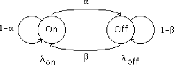
Figure 1: Interrupted Poisson Process source model.
In this section we discuss the approach described by Yuang [2]. Yuang uses a discrete-time Interrupted Poisson Process (IPP) to model packet interarrivals.

Figure 1: Interrupted Poisson Process source model.
More accurately, the channel model is a discrete-time IPP. The channel is either in the state
on or the state off. In the on state, a packet arrives in each
time slot according to a Bernoulli distribution with parameter
![]() . In the off state, packets do not
arrive. The channel transitions from good
to bad with probability
. In the off state, packets do not
arrive. The channel transitions from good
to bad with probability ![]() , and from bad to good with probability
, and from bad to good with probability ![]() . Thus, the
transitions in the source model are given by
. Thus, the
transitions in the source model are given by
Now that packet arrivals are characterized, we continue by modeling the state of the buffer, with another Markov model. In this model, each state corresponds to a level of buffer fullness. State 5, for instance, signifies that there are five packets in the buffer.

Figure 2: Markov model of buffer fullness
Figure 2 illustrates. In figure 2, state transitions occur each time a packet is removed from the buffer for playout. If the buffer is in state i and no packets arrive during the packet playout period, the buffer will transition to state i-1. If one packet arrives it will remain in state i, if two arrive it will transition to i+1 and so on. The key now is to find these transition probabilities.
Let ![]() , where
, where ![]() ,
, ![]() ,
,
![]() be the probability that in t time slots k packets arrive and
the channel ends in state s, given that the model begins
in state r (M is the number of time slots per frame period). Define
be the probability that in t time slots k packets arrive and
the channel ends in state s, given that the model begins
in state r (M is the number of time slots per frame period). Define

The following expression allows the calculation of an arbitrary ![]()
![]()
It sums the probabilities of all the possible outcomes that give k packets arriving in t slots, during which time the channel transitions from r to s. Now we can use these packet arrival distributions to find the transition probabilities from one buffer state to another. Suppose that it takes t time slots to play out a frame. The probability that k packets arrive in time, t is given by
Yuang assumes that the channel state probabilities are given by
the steady-state distribution ![]() ,
,
![]()
Using these stationary distributions of the channel state and allowing the length of time, t, between frame departures to be a function, f(i) of the buffer fullness for an adaptive scheme, we derive the transition probabilities from equation 4:
Note that we have not specified the i = 0 case here. The zero state corresponds to a buffer underflow. In later sections of the paper we will vary how these transition probabilities from state zero are handled to suit our needs.