Digital Image Processing
Home
Class Information
Class Schedule
Handouts
Projects Win 2018/19
Projects Win 2017/18
Projects Aut 2016/17
Projects Aut 2015/16
Projects Spr 2014/15
Projects Spr 2013/14
Projects Win 2013/14
Projects Aut 2013/14
Projects Spr 2012/13
Projects Spr 2011/12
Projects Spr 2010/11
Projects Spr 2009/10
Projects Spr 2007/08
Projects Spr 2006/07
Projects Spr 2005/06
Projects Spr 2003/04
Projects Spr 2002/03
Test Images
MATLAB Tutorials
Android Tutorials
SCIEN
BIMI
Final Project for Spring 2003-2004
Automatic Detection of Defects in Photomask Images
At various stages in the IC manufacturing process defects need to be inspected to ensure process integrity. One key element of this is the detection of defects in photomasks (also referred to as “masks”), which are photographic quartz or glass plates that contain the circuit patterns used in the silicon-chip fabrication process. In order to have an IC production chain that has a sufficiently high yield, it is essential that any defects that arise in photomasks be detected, as the quality of the resulting ICs can only be as good as that of the photomask. In this sense, the quality of the photomask functions as one of several quality bottlenecks in the manufacturing process. A defect can be any flaw affecting the geometry of the resulting circuit. This includes chrome where it was not specified to be (spots, extensions, bridging, etc.) or undesired clear areas (pin holes, “mouse bites”, clear breaks, etc.). A defect can cause the circuit to either not function properly or at all. As no manufacturing process can ever be perfect, chip designers give a certain error tolerance to the fabrication plant and any defects that go beyond these specifications result in an unusable photomask.
Mask defect detection typically takes one of two forms:
· Die-to-die (D:D) – This method compares two optical images from differed dice on the same mask, where the two dice are designed to have the same pattern. Since in most cases the probability of having the same defect occur at the same location in different dice is negligible, an agreement between the two images is considered to indicate a good pattern. A disagreement is therefore considered to be a defect.
· Die-to-database (D:DB) – In this method, a captured optical image of the photomask is compared to a rendered image from the intended design pattern database, which functions as the ideal correct model. In this sense D:DB is similar to D:D except that the other die is actually a perfectly rendered target image.


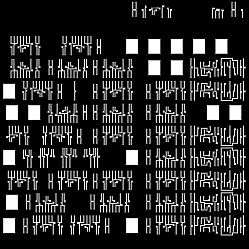
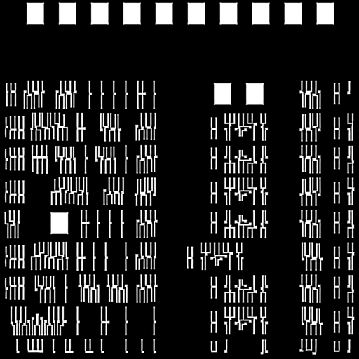
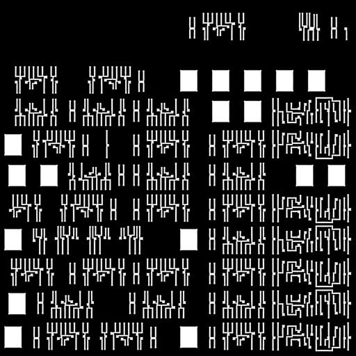
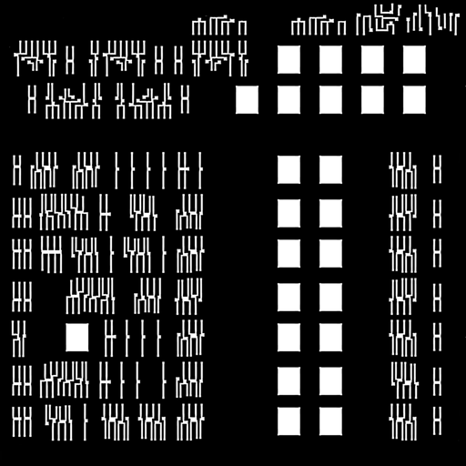
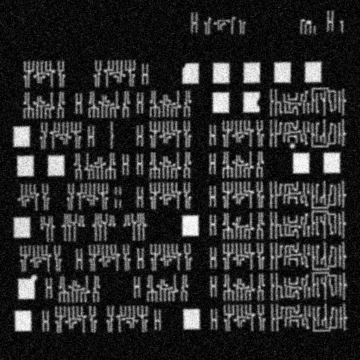
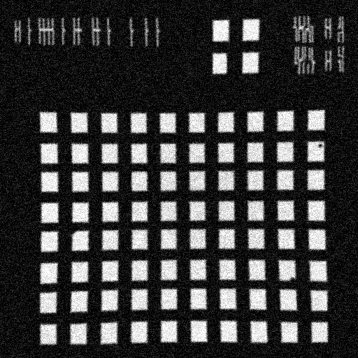
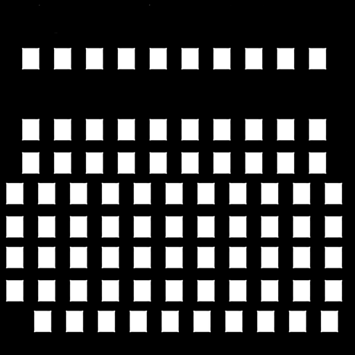
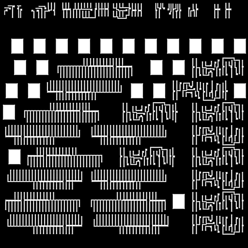
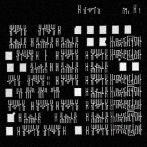
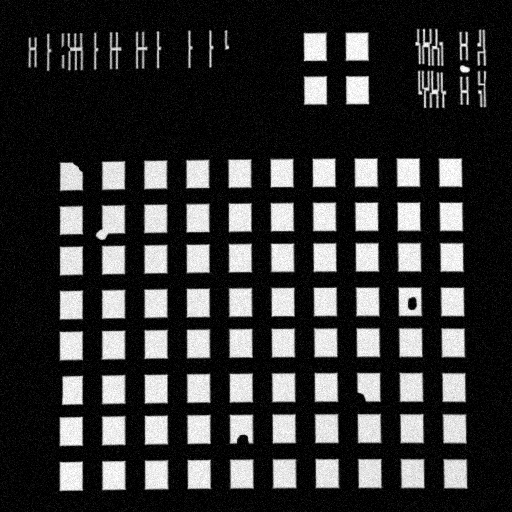
Figure 1: D:DB Inspection Figure 2: D:D Inspection
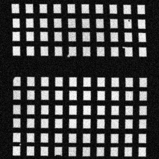
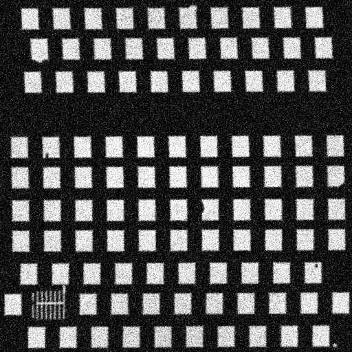
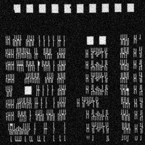
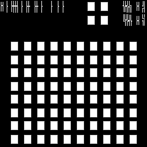
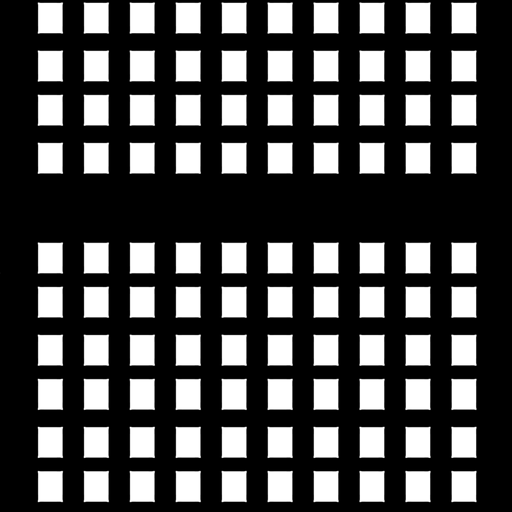
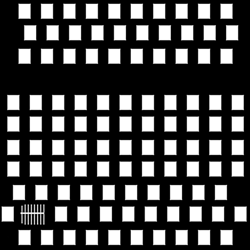
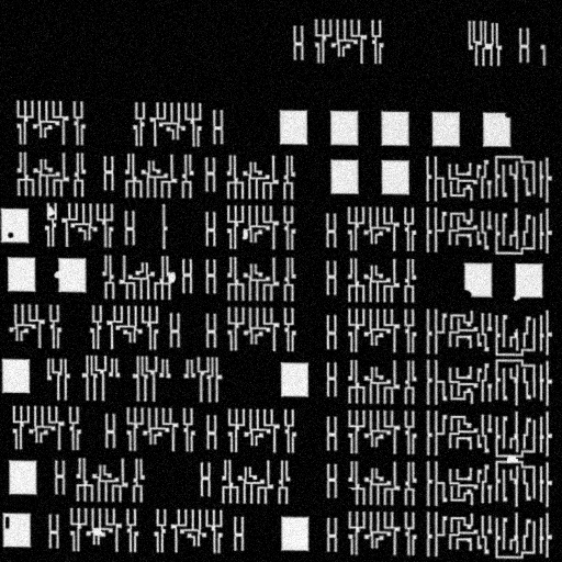
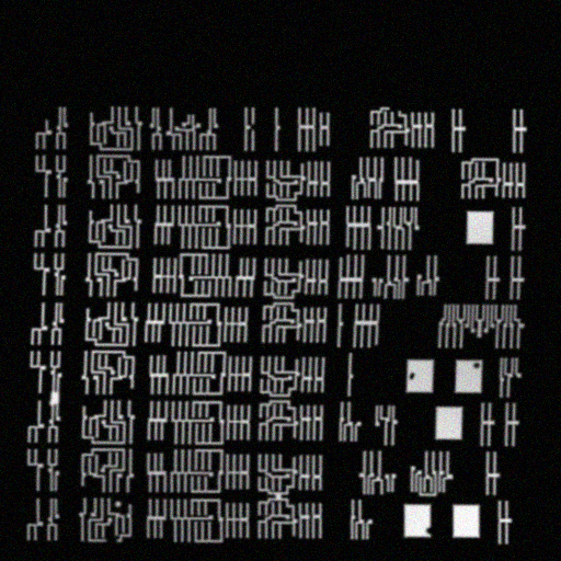
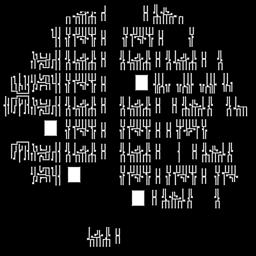
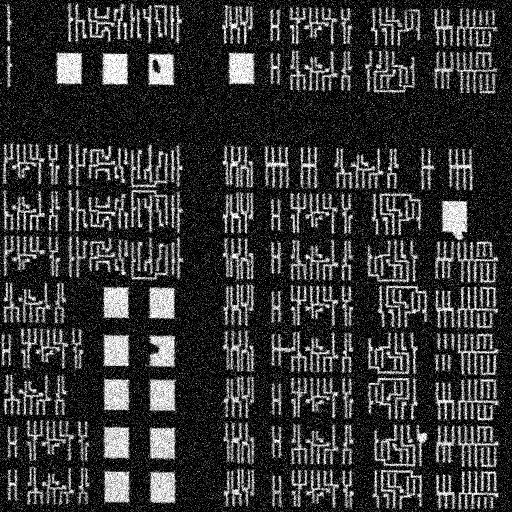
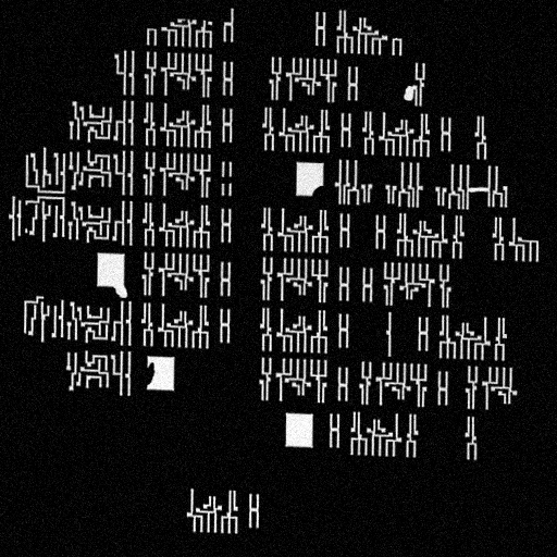
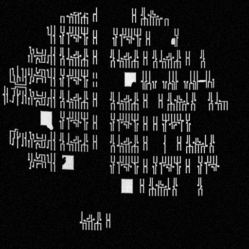
In this project, your goal is to develop an efficient automatic defect detection algorithm according to the D:DB method that can applied to photomask images that have been corrupted and distorted in various ways. As inputs to your algorithm you are given two images: one representing the database image (the template for a correct photomask) and a noisy and distorted image representing an actual photomask that you are inspecting for the presence of defects. Noise and distortion can take the form of warping, shifting, additive noise, linear filtering, rotating, shading, and resizing. The number of defects varies from case to case. Given these two images, your algorithm should produce as its output both the number of detected defects as well as the coordinates of the defects detected, if any. Each detected defect should be specified by its associated coordinates only once. Because defects will always be larger than a single pixel, your algorithm will be considered correct if it is able to return the coordinates of one (and only one) of the pixels associated with a given defect. Errors to be avoided are misses, false alarms, and multiple hits.
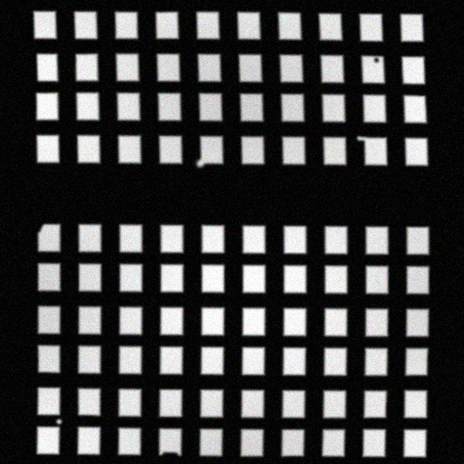
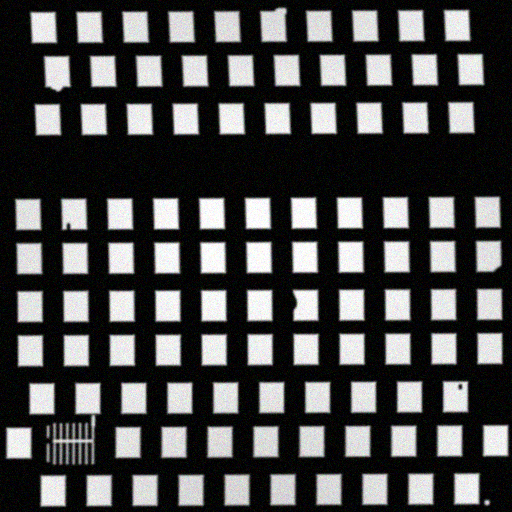
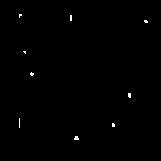
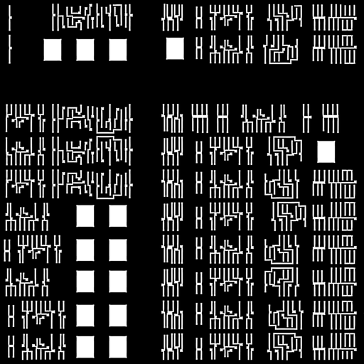
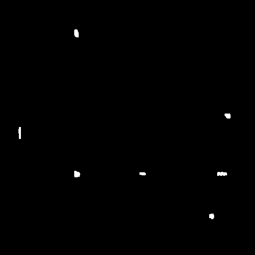
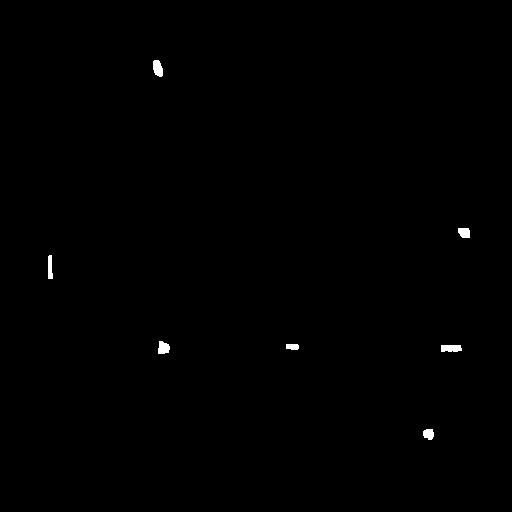
To assist you in developing your algorithms, 10 sets of training images are provided. Each set will consist of three images: the template (correct) database image, the distorted and noisy image to inspect, and an error mask image indicating in the frame of reference of the distorted image the location of pixels that are parts of defects. By using the error mask image you will both know the location of the defects in the training images and know what is considered to be a defect for this project. In all cases, defects will be clear and unambiguous.
While reliability of your algorithm is very important, computational efficiency should be considered as well. As described below, while accuracy will be the primary criterion by which you will be graded, in the cases of equally accurate algorithms performance time will be used as the tie-breaker.
| Set 1 | Set 2 | Set 3 | Set 4 | Set 5 | Set 6 | Set 7 | Set 8 | Set 9 | Set 10 | |
| template database image | link | link | link | link | link | link | link | link | link | link |
| image to be inspected | link | link | link | link | link | link | link | link | link | link |
| mask image | link | link | link | link | link | link | link | link | link | link |
The images below are a training set of "easy" images. These can be used to aid algorithm development. However, expect the test set to contain more difficult images.
| Set 1n | Set 2n | Set 3n | Set 4n | Set 5n | Set 6n | Set 7n | Set 8n | Set 9n | Set 10n | |
| template database image | link | link | link | link | link | link | link | link | link | link |
| image to be inspected | link | link | link | link | link | link | link | link | link | link |
| mask image | link | link | link | link | link | link | link | link | link | link |
There are three major steps in the detection project:
(1). Design and implement your routine in MATLAB based on the provided training image sets.
(2). Test your routines with the training image sets by the evaluation program.
(3). Performance of your routine will be tested with a test image set by the same evaluation program.
Each step is explained in detail below.
(1). Your Defect Detection Routine:
Format
Your main routine has to be in this format: function defects = defect_detection(imgDB_filename, imgD_filename).
INPUT: imgDB_filename and imgD_filename are filenames of the template database image and the image to be inspected in BMP format respectively. For instance, for the first training image set imgDB_filename and imgD_filename should be 'training_1_DB.bmp' and 'training_1_D.bmp' respectively.
OUTPUT: a N-by-2 matrix named 'defects' containing the coordinates of each detected defect
-- N is the number of detects you’ve detected
-- defects(:,1) contains the detected vertical coordinates (row index of the image matrix)
-- defects(:,2) contains the detected horizontal coordinates (column index of the image matrix)
You can call other sub-routines under this main routine. The main routine serves as the interface with our evaluation program. In the final test with the test image set, we'll call your main routine in the evaluation program by defects = defect_detection(xxx, xxx).
Time-Limit
The time-limit for your routines is 10 minutes (when running on a ISE lab machine with most resource available). You should monitor the execution time and output the results by that time-limit. Our evaluation program can check if you are within the time-limit only after your routine is terminated. In other words, you need to make sure you finish your routine in time and return the proper result.
You might want to start your routine with a rough estimation, and then check the time remaining. If there is a certain amount of time left, refine your estimation. Otherwise, output what you’ve got and terminate your routine. You can also down-sample the image to reduce the amount of computation required. However, this down-sampling process should be part of your own routine. When we test your algorithm, the test image set will be in the same resolution as the training image sets posted on the web.
(2). Evaluation Program (evaluate.m)
Format:
[detectScore, numHit, numRepeat, numFalsePositive, runTime] = ...
evaluate(imgDB_filename, imgD_filename, mask_filename)
INPUT:
1. imgDB_filename: filename of the template database image in BMP format
2. imgD_filename: filename of the image to be inspected in BMP format
3. mask_filename: filename of the mask image in BMP format
OUTPUT:
1. detectScore = numHit - numRepeat - numFalsePositive (from output 2,3,4)
2. numHit = number of defects successfully detected
3. numRepeat = number of defects repeatedly detected
4. numFalsePositive = number of cases where a non-defect is reported
5. runTime = run time of your defect detection routine
Example:
[detectScore, numHit, numRepeat, numFalsePositive, runTime] = ...
evaluate('training_1_DB.bmp', 'training_1_D.bmp', 'training_1_mask.bmp')
(3). Performance Criterion
The performance of your routine is judged by outputs of the evaluation program. There are two criterions:
(a). Detection Score:
The detectScore from the evaluation program indicates your detection accuracy.
(b). Run-Time:
You need to make sure your run-time is within the given time limit (10 minutes). Otherwise, we might need to terminate your routine without getting any result. In addition, while detection accuracy will be the primary criterion by which you will be graded, in the cases of equally accurate algorithms the run-time will be used as the tie-breaker.
5. Testing Image Sets and Final Evaluation Results
| Set 1 | Set 2 | Set 3 | Set 4 | Set 5 | Set 6 | Set 7 | Set 8 | |
| template database image | link | link | link | link | link | link | link | link |
| image to be inspected | link | link | link | link | link | link | link | link |
| mask image | link | link | link | link | link | link | link | link |
In evaluating your algorithms, a total of eight image sets were used. These were based on two different underlying circuit diagrams and varied with respect to the level of both the warping/distortion and additive noise that the images were subjected to. Projects are ranked below, listing the total score (maximum of 60 points) and the average run time. Note that projects were ranked first according to accuracy (reflected by the “program score”) and then ranked according to the average run time in the case of a tie. Although not used in the rankings, program report scores are also given below (maximum of 100 points). For the program score and average time metrics, “N/A” denotes the case of a student’s program failing to run during our tests.
SUID Program Score Average Time (sec.) Report Score
5282348 55 12.8 90
5250843 55 39.1 87
5251589 55 174.8 86
5282208 53 13.2 92
5249821 52 73.9 90
5282347 51 27.9 95
3357936 50 12.0 85
5239433 50 25.9 89
5246123 50 28.7 95
5135197 50 35.2 93
5273677 48 18.2 85
5239460 47 35.3 90
5246741 46 7.9 78
5249584 46 76.1 88
4365672 45 269.3 84
5157803 42 6.3 85
5251106 41 43.6 88
5144745 41 65.8 86
4799482 40 41.6 92
5156136 40 286.4 78
5249039 40 289.1 84
5223781 40 303.3 86
5244480 39 8.8 84
5151400 38 58.8 81
5244703 37 77.4 86
5238838 36 108.1 91
5250977 35 13.6 84
5250783 35 54.5 90
5241126 35 54.7 70
5153329 35 84.3 82
5248972 34 67.2 87
5249709 34 148.6 89
5239486 31 14.7 93
5250957 31 17.8 87
4842597 30 7.7 88
5168071 29 6.3 72
5251160 28 39.3 84
4909958 28 135.2 84
5233415 27 108.1 88
4673745 27 254.3 81
5249012 26 29.3 92
5249022 26 1042.4 80
5248816 26 1048.6 83
5246803 25 7.5 79
4766630 24 44.8 85
5230896 23 13.0 84
5264635 23 15.2 79
5252465 23 47.8 86
5221975 21 423.1 90
5121837 20 34.5 83
5157887 18 337.5 80
5245903 17 21.4 79
4833109 15 74.2 85
5242600 15 79.1 85
5248194 13 140.9 83
5246064 10 32.5 95
5111139 12 190.6 83
5235104 11 70.9 80
5113339 10 294.4 87
5104960 08 368.9 74
4924262 07 32.3 86
5244057 07 41.1 87
5103372 06 31.6 91
5251323 01 38.4 82
5153772 01 159.5 80
5247553 01 280.2 82
4385035 0 0.1 78
3799236 0 12.5 90
5195553 0 19.0 77
5119910 0 23.0 74
5114544 0 33.0 77
5163081 0 137.8 88
5157767 0 343.1 82
5252124 0 715.9 74
5233395 N/A N/A 80
4788030 N/A N/A 0
4883724 N/A N/A 77
4609897 N/A N/A 0